

About Manuel Amunategui
Data scientist with over 20-years experience in the tech industry, MAs in Predictive Analytics and
International Administration, co-author of Monetizing Machine Learning and VP of Data Science at SpringML.
From consulting in machine learning, healthcare modeling, 6 years on Wall Street in the financial industry, and 4 years at Microsoft, I feel like I’ve seen it all. And this has opened my eyes to the huge gap in educational material on applied data science. Like I say:
It just ain’t real 'til it reaches your customer’s plate
I am a startup advisor and available for speaking engagements with companies and schools on topics around building and motivating data science teams, and all things applied machine learning.
Reach me at amunategui@gmail.com


|

What-if Roadmap - Assessing Live Opportunities and their Paths to Success or Failure
Practical walkthroughs on machine learning, data exploration and finding insight.

Resources
In the pursuit of actionable insights, we can use historical closed opportunities that are similar to open ones and analyze what made one win and another lose. This doesn’t necessarily have to be sales data, it can be anything that hasn’t reached some outcome or end point - where there is still some unknown factor.
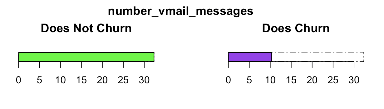
We’ll use the built-in data set supplied with the C5.0 R library, called Customer Churn. As the name implies, the data contains customer information and usage records from a phone company including whether the customer churned or not. Here is one of the “what ifs”, lack of voice mail usage may indicate a churning customer.
The R statistical programming language has a function called stringdist which:
‘Implements an approximate string matching version of R’s native ’match’ function’.
It contains a large set of matching approaches:
- osa Optimal string aligment, (restricted Damerau-Levenshtein distance)
- lv Levenshtein distance
- dl Full Damerau-Levenshtein distance
- hamming Hamming distance
- lcs Longest common substring distance
- qgram q-gram distance
- cosine cosine distance between q-gram profiles
- jaccard Jaccard distance between q-gram profiles
- jw Jaro, or Jaro-Winker distance
- soundex Distance based on soundex encoding
In this example we are using the jaccard matching approach.
An Example using a Toy Dataset
# install.packages('dplyr')
library(dplyr)
##
## Attaching package: 'dplyr'## The following objects are masked from 'package:stats':
##
## filter, lag## The following objects are masked from 'package:base':
##
## intersect, setdiff, setequal, union# install.packages('C50')
library(C50)
data(churn)
churn_data <- churnTrain
outcome_name <- 'churn'
In our toy example, we take the first row as our hypothetical live case, and consider all other rows as closed, historical opportunities (in this case whether or not a customer has churned)
# pick focus customer - from which to find matching cases from your historical data
live_row <- churn_data[1,]
historical_df <- churn_data[-1,]
Now that we have two data sets, we apply the stringdist function to get our distance metrics from our historical data in comparison to our picked hypothetical live customer.
# install.packages('stringdist')
library(stringdist)
# hide outcome variable as it is unknown in a live set
similar_metrics <- Reduce(`+`,Map(stringdist, dplyr::select(historical_df, -churn),
                                      dplyr::select(live_row, -churn),
                                      method='jaccard'))

head(similar_metrics)
## [1] 9.166667 13.911905 15.102381 12.379762 14.668723 12.484199Hi there, this is Manuel Amunategui- if you're enjoying the content, find more at ViralML.com
A good next step is to add our distance metrics back to the historical data set and pull the closest matches with our focus row for both positive and negative outcomes.
# print focus row for comparaisoin
live_row
## state account_length area_code international_plan voice_mail_plan
## 1 KS 128 area_code_415 no yes
## number_vmail_messages total_day_minutes total_day_calls total_day_charge
## 1 25 265.1 110 45.07
## total_eve_minutes total_eve_calls total_eve_charge total_night_minutes
## 1 197.4 99 16.78 244.7
## total_night_calls total_night_charge total_intl_minutes total_intl_calls
## 1 91 11.01 10 3
## total_intl_charge number_customer_service_calls churn
## 1 2.7 1 no# assign metrics back to historical data set
historical_df$similar <- similar_metrics
# set number of similar rows needed per outcome
rows_to_collect <- 1
# get first similar item that has positive outcome
historical_df %>% dplyr::filter(churn == 'yes') %>%
dplyr::arrange(similar) %>% head(rows_to_collect) ## state account_length area_code international_plan voice_mail_plan
## 1 KS 170 area_code_415 no yes
## number_vmail_messages total_day_minutes total_day_calls total_day_charge
## 1 42 199.5 119 33.92
## total_eve_minutes total_eve_calls total_eve_charge total_night_minutes
## 1 135 90 11.48 184.6
## total_night_calls total_night_charge total_intl_minutes total_intl_calls
## 1 49 8.31 10.9 3
## total_intl_charge number_customer_service_calls churn similar
## 1 2.94 4 yes 9.446429# get first similar item that has negative outcome
historical_df %>% dplyr::filter(churn == 'no') %>%
dplyr::arrange(similar) %>% head(rows_to_collect) ## state account_length area_code international_plan voice_mail_plan
## 1 AR 89 area_code_415 no yes
## number_vmail_messages total_day_minutes total_day_calls total_day_charge
## 1 25 215.1 140 36.57
## total_eve_minutes total_eve_calls total_eve_charge total_night_minutes
## 1 197.4 69 16.78 162.1
## total_night_calls total_night_charge total_intl_minutes total_intl_calls
## 1 117 7.29 10.6 10
## total_intl_charge number_customer_service_calls churn similar
## 1 2.86 1 no 7.621429
As we are after insights that are ‘actionable’, we need to look at our features and remove those that don’t lend itself to ‘action’, like geographic markers. Let’s remove ‘State’ and ‘Area Code’.
# state and area_code not of big interest in terms of affectable actions
live_row %>% dplyr::select(-state, -area_code) -> live_row
historical_df %>% dplyr::select(-state, -area_code) -> historical_df


historical_df$similar <- Reduce(`+`,Map(stringdist, dplyr::select(historical_df, -churn),
                                        dplyr::select(live_row, -churn),
                                        method='jaccard'))
## Warning in mapply(FUN = f, ..., SIMPLIFY = FALSE): longer argument not a
## multiple of length of shorter# set number of similar rows needed per outcome
rows_to_collect <- 3
# get first similar item that has positive outcome
historical_df %>% dplyr::filter(churn == 'yes') %>%
dplyr::select(-churn) %>%
dplyr::arrange(similar) %>% head(rows_to_collect) -> positive_historical_df
# get first similar item that has negative outcome
historical_df %>% dplyr::filter(churn == 'no') %>%
dplyr::select(-churn) %>%
dplyr::arrange(similar) %>% head(rows_to_collect) -> negative_historical_df
Correlations - Finding Features Moving in Opposite Direction
We’re almost there, now that we have our closest top positive and negative similar cases, let’s take a look at what features were the most inverslely correlated. We’ll use the cor function to find the features moving in opposite direciton as these may offer insight into what can be done to understand and affect a positive outcome.
# find extreme examples best portraying different directions ----------------------------
diverging_features <- c()
order_ids <- c()
average_neg <- c()
average_pos <- c()
for (col_id in seq(ncol(positive_historical_df))) {

  positive_historical_df[,col_id]  <- as.numeric(positive_historical_df[,col_id])
  negative_historical_df[,col_id]  <- as.numeric(negative_historical_df[,col_id])

  similar_cor <- (cor(positive_historical_df[,col_id], negative_historical_df[,col_id]))
  if (!is.na(similar_cor) && (similar_cor < -0.2)) {
    print(names(positive_historical_df)[col_id])
    diverging_features <- c(diverging_features, names(positive_historical_df)[col_id])
    order_ids <- c(order_ids, col_id)


    # plot as vertical bar chart
    pos_df <- data.frame('Opp_ID'=paste0('Opp_ID_',seq(nrow(positive_historical_df))),
                         'Value'=(positive_historical_df[,col_id]),
                         'Influence'='Positive')
    neg_df <-  data.frame('Opp_ID'=paste0('Opp_ID_',seq(nrow(negative_historical_df))),
                          'Value'=(negative_historical_df[,col_id]),
                          'Influence'='Negative')

    # flip negative scale for side-by-side plotting
    pos_df$Value <- as.numeric(pos_df$Value)
    neg_df$Value <- as.numeric(neg_df$Value) * -1


    par(mfrow=c(1,2))
    max_xlim <- max(max(abs(neg_df$Value)), max(abs(pos_df$Value)))
    barplot(neg_df$Value, main="Negative Trend", horiz=TRUE, xlim=c((max_xlim * -1),0),
            col='red', border = 1, xaxt='n')
    box(lty = '1373', col = 'black')
    barplot(pos_df$Value, main="Positive Trend", horiz=TRUE, xlim=c(0, max_xlim), col='blue',
            beside=FALSE, names.arg=pos_df$Opp_ID,las=1, xaxt='n')
    box(lty = '1373', col = 'black')
    title(paste("Doctor Trending\n",names(positive_historical_df)[col_id]), outer=TRUE)

    # return conclusion for opportunity ID
    average_neg <- c(average_neg, mean(abs(neg_df$Value)))
    average_pos <- c(average_pos, mean(abs(pos_df$Value)))

  }
}
## Warning in cor(positive_historical_df[, col_id], negative_historical_df[, :
## the standard deviation is zero
## Warning in cor(positive_historical_df[, col_id], negative_historical_df[, :
## the standard deviation is zero## [1] "number_vmail_messages"
## [1] "total_day_minutes"
## [1] "total_day_charge"
## [1] "total_eve_minutes"
## [1] "total_eve_charge"
## [1] "total_intl_calls"## Warning in cor(positive_historical_df[, col_id], negative_historical_df[, :
## the standard deviation is zero
As with most ‘advanced analytics’ results aren’t simple and/or easy - otherwise it would be considered simple and your client would most likely already know about it. It is critical to look at the whole picture, look for outliers and significance, etc.
recommendations <-  data.frame(diverging_features = diverging_features,
                               order_ids = order_ids,
                               average_neg = average_neg,
                               average_pos = average_pos)

# present cases of interest
for (case_id in seq(nrow(recommendations))) {
  print(case_id)

  # what if both values are negatigve, or one of each?

  par(mfrow=c(1,2))
  max_xlim <- max(max(abs(recommendations$average_pos[case_id])), max(abs(recommendations$average_neg[case_id])))
  barplot(recommendations$average_neg[case_id], main="Does Not Churn", horiz=TRUE, xlim=c(0, max_xlim),
          col='green', border = 1)
  box(lty = '1373', col = 'black')

  barplot(recommendations$average_pos[case_id], main="Does Churn", horiz=TRUE, xlim=c(0, max_xlim), col='purple',
          beside=FALSE) #, names.arg=recommendations$diverging_features[case_id],las=1)

  box(lty = '1373', col = 'black')
  title(paste("Doctor Trending\n",recommendations$diverging_features[case_id]), outer=TRUE)

}
## [1] 1
## [1] 2
## [1] 3
## [1] 4
## [1] 5
## [1] 6
Manuel Amunategui - Follow me on Twitter: @amunategui
Thanks again for the artwork, Lucas!!