

About Manuel Amunategui
Data scientist with over 20-years experience in the tech industry, MAs in Predictive Analytics and
International Administration, co-author of Monetizing Machine Learning and VP of Data Science at SpringML.
From consulting in machine learning, healthcare modeling, 6 years on Wall Street in the financial industry, and 4 years at Microsoft, I feel like I’ve seen it all. And this has opened my eyes to the huge gap in educational material on applied data science. Like I say:
It just ain’t real 'til it reaches your customer’s plate
I am a startup advisor and available for speaking engagements with companies and schools on topics around building and motivating data science teams, and all things applied machine learning.
Reach me at amunategui@gmail.com


|

Convolutional Neural Networks And Unconventional Data - Predicting The Stock Market Using Images
Practical walkthroughs on machine learning, data exploration and finding insight.
On YouTube:

NOTE: Full source code at end of the post has been updated with latest Yahoo Finance stock data provider code along with a better performing covnet. Refer to pandas-datareader docs if it breaks again or for any additional fixes.
This post is about taking numerical data, transforming it into images and modeling it with convolutional neural networks. In other words, we are creating synthetic image-representation of quantitative data, and seeing if a CNN brings any additional modeling understanding, accuracy, a boost via ensembling, etc. CNN’s are hyper-contextually aware - they know what’s going on above, below, to the right and to the left, even what is going on in front and behind if you use image depth.
The genesis for this idea came from bridging the ‘retail’ trader, a predominantly visual approach, to the ‘quant/HFT’ trader, a numerical one. I have been a professional on both sides for many years. Retail trading looks at support/resistance levels, moving averages, chart patterns, new highs/lows, etc. - mostly visual patterns based off of stock charts. The quantitative trader may use order flow, order depth, imbalances between exchanges, complex hedging, delta-neutral synthetic products, Black-Scholes pricing estimates, binomial distributions, etc. - all numerical data.
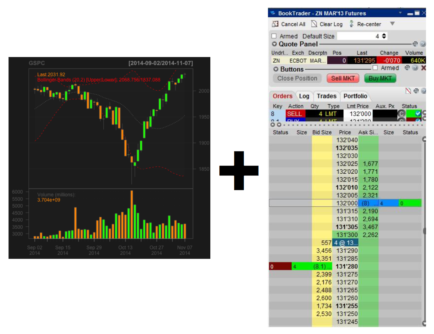
By feeding stock charts into convolutional networks, you are blending both visual and quantitative trading styles. Here we will create synthetic market charts, thousands of them, and train CNNs to find patterns for us.
Note on data and trading system: first off, this is only for education and entertainment, not for actual trading! We’ll use Google finance to pull data - it gives only one year’s worth of historical data. I would recommend using Quandl or another service to access a lot more financial data for longer historical periods.
Creating Synthetic Images
An important advantage of working with images is that you can load them up with many features. Think of the following dataset of end-of-day GOOG, you could very easily split an image into four quadrants and add the Open in one quadrant, the High in another, and so on. That's four time-series in one image!
import pandas_datareader as pdr
stock_data = pdr.get_data_google('GOOG')
stock_data.head()
Out[116]:
Open High Low Close Volume
Date
2016-10-31 795.47 796.86 784.00 784.54 2427284
2016-11-01 782.89 789.49 775.54 783.61 2406356
2016-11-02 778.20 781.65 763.45 768.70 1918414
2016-11-03 767.25 769.95 759.03 762.13 1943175
2016-11-04 750.66 770.36 750.56 762.02 2134812
Here, we’re going to take 20 day data segments (20 consecutive trading periods) and split our image into two halves. The top half with the closing price segments overlaid by a rolling average of the same.
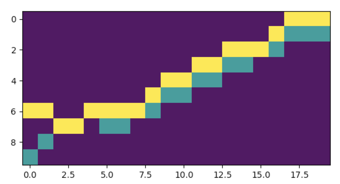
The bottom half will hold a derived market indicator made of the Close minus the Open.
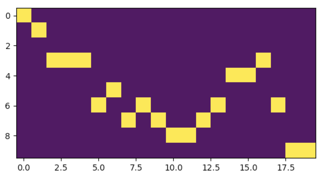
When you splice them together, you get the following square matrix. That's it, there's our image - a complex time-series representation of various price action data for how many periods you choose (40 in the below example):
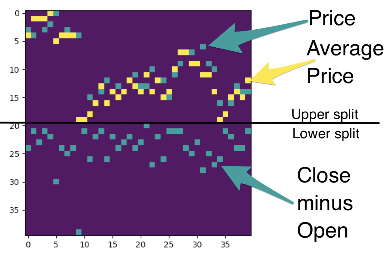
As you can see, it contains the same type of data you would see in a conventional stock chart - price and moving averages on top and indicators on the bottom. The difference here is that we are modeling the data, so we need a lot more than just one chart, we need millions of them. Here is a patchwork of thousands of them:

Hi there, this is Manuel Amunategui- if you're enjoying the content, find more at ViralML.com
 Getting End-Of-Day Market Data For Dow 30 Stocks & Building Image Segments
We’ll use pandas_datareader to pull financial data from Google. We pull 20-day segments and scale it between 0 and 10. This creates a concise range between all Dow 30 stocks and emulates an actual real stock chart where the bottom of the chart captures the minimum price of the segment and the top, the maximum.
To help stabilize the price and give us a predictive boost, we smooth the closing price down by using a 3-day moving average. We overlay a 6-day moving average over it as well (as shown in the above charts). You are encouraged to play around with these moving average values, and even trying without any averages as you would in a day-trading scenario (but definitely get more data for longer periods of time to give the model a better understanding of market environments).
We need to create our outcome label, here we will predict whether the 3-day moving average will be above the 6-day moving average, implying an up day - vice-versa for down days.
import time
import datetime
import pandas as pd
import numpy as np
import pandas_datareader as pdr
import matplotlib.pyplot as plt


def scale_list(l, to_min, to_max):

    def scale_number(unscaled, to_min, to_max, from_min, from_max):
        return (to_max-to_min)*(unscaled-from_min)/(from_max-from_min)+to_min

    if len(set(l)) == 1:
        return [np.floor((to_max + to_min)/2)] * len(l)
    else:
        return [scale_number(i, to_min, to_max, min(l), max(l)) for i in l]


STOCKS = ['AAPL', 'AXP', 'BA', 'CAT', 'CSCO', 'CVX', 'DD', 'DIS', 'GE', 'GS', 'HD', 'IBM', 'INTC', 'JNJ', 'JPM', 'KO', 'MCD', 'MMM', 'MRK', 'MSFT', 'NKE', 'PFE', 'PG', 'UNH', 'UTX', 'V', 'VZ', 'WMT', 'XOM']


TIME_RANGE = 20
PRICE_RANGE = 20
VALIDTAION_CUTOFF_DATE = datetime.date(2017, 7, 1)

# split image horizontally into two sections - top and bottom sections
half_scale_size = int(PRICE_RANGE/2)

live_symbols = []
x_live = None
x_train = None
x_valid = None
y_train = []
y_valid = []

for stock in STOCKS:
    print(stock)

    # build image data for this stock
    stock_data = pdr.get_data_google(stock)
    stock_data['Symbol'] = stock
    stock_data['Date'] = stock_data.index
    stock_data['Date'] = pd.to_datetime(stock_data['Date'], infer_datetime_format=True)
    stock_data['Date'] = stock_data['Date'].dt.date
    stock_data = stock_data.reset_index(drop=True)

    # add Moving Averages to all lists and back fill resulting first NAs to last known value
    noise_ma_smoother = 3
    stock_closes = pd.rolling_mean(stock_data['Close'], window = noise_ma_smoother)
    stock_closes = stock_closes.fillna(method='bfill')
    stock_closes =  list(stock_closes.values)
    stock_opens = pd.rolling_mean(stock_data['Open'], window = noise_ma_smoother)
    stock_opens = stock_opens.fillna(method='bfill')
    stock_opens =  list(stock_opens.values)

    stock_dates = stock_data['Date'].values

    close_minus_open = list(np.array(stock_closes) - np.array(stock_opens))

    # lets add a rolling average as an overlay indicator - back fill the missing
    # first five values with the first available avg price
    longer_ma_smoother = 6
    stock_closes_rolling_avg = pd.rolling_mean(stock_data['Close'], window = longer_ma_smoother)
    stock_closes_rolling_avg = stock_closes_rolling_avg.fillna(method='bfill')
    stock_closes_rolling_avg =  list(stock_closes_rolling_avg.values)

    for cnt in range(4, len(stock_closes)):
        if (cnt % 500 == 0): print(cnt)

        if (cnt >= TIME_RANGE):
            # start making images
            graph_open = list(np.round(scale_list(stock_opens[cnt-TIME_RANGE:cnt], 0, half_scale_size-1),0))
            graph_close_minus_open = list(np.round(scale_list(close_minus_open[cnt-TIME_RANGE:cnt], 0, half_scale_size-1),0))

            # scale both close and close MA toeghertogether
            close_data_together = list(np.round(scale_list(list(stock_closes[cnt-TIME_RANGE:cnt]) +
                list(stock_closes_rolling_avg[cnt-TIME_RANGE:cnt]), 0, half_scale_size-1),0))
            graph_close = close_data_together[0:PRICE_RANGE]
            graph_close_ma = close_data_together[PRICE_RANGE:]

            outcome = None
            if (cnt < len(stock_closes) -1):
                outcome = 0
                if stock_closes[cnt+1] > stock_closes_rolling_avg[cnt+1]:
                    outcome = 1

            blank_matrix_close = np.zeros(shape=(half_scale_size, TIME_RANGE))
            x_ind = 0
            for ma, c in zip(graph_close_ma, graph_close):
                blank_matrix_close[int(ma), x_ind] = 1
                blank_matrix_close[int(c), x_ind] = 2
                x_ind += 1

            # flip x scale dollars so high number is atop, low number at bottom - cosmetic, humans only
            blank_matrix_close = blank_matrix_close[::-1]

            # store image data into matrix DATA_SIZE*DATA_SIZE
            blank_matrix_diff = np.zeros(shape=(half_scale_size, TIME_RANGE))
            x_ind = 0
            for v in graph_close_minus_open:
                blank_matrix_diff[int(v), x_ind] = 3
                x_ind += 1
            # flip x scale so high number is atop, low number at bottom - cosmetic, humans only
            blank_matrix_diff = blank_matrix_diff[::-1]

            blank_matrix = np.vstack([blank_matrix_close, blank_matrix_diff])

            if 1==2:
                # graphed on matrix
                plt.imshow(blank_matrix)
                plt.show()

                # straight timeseries
                plt.plot(graph_close, color='black')
                plt.show()

            if (outcome == None):
                # live data
                if x_live is None:
                    x_live =[blank_matrix]
                else:
                    x_live = np.vstack([x_live, [blank_matrix]])
                live_symbols.append(stock)

            elif (stock_dates[cnt] >= VALIDTAION_CUTOFF_DATE):
                # validation data
                if x_valid is None:
                    x_valid = [blank_matrix]
                else:
                    x_valid = np.vstack([x_valid, [blank_matrix]])
                y_valid.append(outcome)

            else:
                # training data
                if x_train is None:
                    x_train = [blank_matrix]
                else:
                    x_train = np.vstack([x_train, [blank_matrix]])
                y_train.append(outcome)
We end up with 3 sets of matrices - one for training, another for validation, and a final one for live data (i.e. the last trading period in our collection where we cannot calculate an outcome as tomorrow hasn’t happened yet).
Modeling with Convolutional Neural Networks
We’re going to use Keras, the higher-level API, to abstract some of the tedious work of building a convolutional network. The model is based on a VGG-like convnet found in the Keras Getting started with the Keras Sequential model’ guide. There are many ways of slicing and dicing such type of model, so definitely experiment away. In a nutshell, we’re using:- Three convolutional layers. The first will detect edges, the second will dig deeper and the third will capture even higher-level features
- A MaxPooling2D layer to reduce dimensionality
- A dropout layer to avoid over-fitting
- And a few dense layers to bring the outcome into focus all the way down to the outcome level
import keras
from keras.models import Sequential
from keras.layers import Dense, Dropout, Flatten
from keras.layers import Conv2D, MaxPooling2D
from keras import backend as K

batch_size = 1000
num_classes = 2
epochs = 20

# input image dimensions
img_rows, img_cols = TIME_RANGE, TIME_RANGE

# add fake depth channel
x_train_mod = x_train.reshape(x_train.shape[0], img_rows, img_cols, 1)
x_valid = x_valid.reshape(x_valid.shape[0], img_rows, img_cols, 1)
input_shape = (TIME_RANGE, TIME_RANGE, 1)

x_train_mod = x_train_mod.astype('float32')
x_valid = x_valid.astype('float32')

print('x_train_mod shape:', x_train_mod.shape)
print('x_valid shape:', x_valid.shape)

y_train_mod = keras.utils.to_categorical(y_train, num_classes)
y_valid_mod = keras.utils.to_categorical(y_valid, num_classes)

model = Sequential()
model.add(Conv2D(64, (5, 5), input_shape=input_shape, activation='relu'))
model.add(Conv2D(32, (3, 3), activation='relu'))
model.add(Conv2D(10, (2, 2), activation='relu'))
model.add(MaxPooling2D(pool_size=(2, 2)))
model.add(Dropout(0.2))
model.add(Flatten())
model.add(Dense(128, activation='relu'))
model.add(Dense(50, activation='relu'))
model.add(Dense(num_classes, activation='softmax'))
# Compile model
model.compile(loss='categorical_crossentropy', optimizer='adam', metrics=['accuracy'])
model.summary()

model.fit(x_train_mod, y_train_mod,
          batch_size=batch_size,
          epochs=epochs,
          verbose=1,
          validation_data=(x_train_mod, y_train_mod))


score = model.evaluate(x_train_mod, y_train_mod, verbose=0)
# print('Test loss:', score[0])
# print('Test accuracy:', score[1])

predictions = model.predict(x_valid)

# run an accuracy or auc test
from sklearn.metrics import roc_curve, auc, accuracy_score

# balance
print('balance', np.mean(y_train_mod[:,1]))
fpr, tpr, thresholds = roc_curve(y_valid_mod[:,1], predictions[:,1])
roc_auc = auc(fpr, tpr)
print('valid auc:',roc_auc)

actuals = y_valid_mod[:,1]
preds = predictions[:,1]
from sklearn.metrics import accuracy_score
print ('Accuracy on all data:', accuracy_score(actuals,[1 if x >= 0.5 else 0 for x in preds]))
balance 0.556956004756
valid auc: 0.600883159876
Accuracy on all data: 0.579686209744
We get an AUC of 0.6, which isn’t bad when predicting the stock market and an accuracy of 57%, so a tad better than the natural balance of the data of 0.55 (so if you picked any at random you would automatically have a 55% success rate). Still this isn’t a lot higher than random. What can we do?
Let's Run With The Best Bets
Well, the model does return probabilities, let’s cherry-pick the higher ones and see how that affects accuracy. Let’s set your prediction threshold to 0.65, meaning that anything below 0.65 will be ignored:
threshold = 0.65
preds = predictions[:,1][predictions[:,1] >= threshold]
actuals = y_valid_mod[:,1][predictions[:,1] >= threshold]
from sklearn.metrics import accuracy_score
print ('Accuracy on higher threshold:', accuracy_score(actuals,[1 if x > 0.5 else 0 for x in preds]))
print('Returns:',len(actuals))
Accuracy on higher threshold: 0.682481751825
Returns: 822Nice! On a subset of 822 predictions, we boosted the accuracy to 68%!!
All Together
import time
import datetime
import pandas as pd
import numpy as np
import matplotlib.pyplot as plt
import pandas_datareader as pdr

def scale_list(l, to_min, to_max):
    def scale_number(unscaled, to_min, to_max, from_min, from_max):
        return (to_max-to_min)*(unscaled-from_min)/(from_max-from_min)+to_min

    if len(set(l)) == 1:
        return [np.floor((to_max + to_min)/2)] * len(l)
    else:
        return [scale_number(i, to_min, to_max, min(l), max(l)) for i in l]


STOCKS = ['AAPL','AXP','BA','CAT','CSCO','CVX','DIS','DWDP','GE','GS','HD','IBM','INTC','JNJ','JPM','KO','MCD','MMM','MRK','MSFT','NKE','PFE','PG','TRV','UNH','UTX','V','VZ','WMT','XOM']

TIME_RANGE = 20
PRICE_RANGE = 20
VALIDTAION_CUTOFF_DATE = datetime.date(2017, 7, 1)

# split image horizontally into two sections - top and bottom sections
half_scale_size = int(PRICE_RANGE/2)

live_symbols = []
x_live = None
x_train = None
x_valid = None
y_train = []
y_valid = []

# xgboost lists
live_data_xgboost = []
validation_data_xgboost = []
train_data_xgboost = []

for stock in STOCKS:
    print(stock)

    # build image data for this stock
    # stock_data = pdr.get_data_google(stock)

    # download dataframe
    stock_data = pdr.get_data_yahoo(stock, start="2016-01-01", end="2018-01-17")

    stock_data['Symbol'] = stock
    stock_data['Date'] = stock_data.index
    stock_data['Date'] = pd.to_datetime(stock_data['Date'], infer_datetime_format=True)
    stock_data['Date'] = stock_data['Date'].dt.date
    stock_data = stock_data.reset_index(drop=True)

    # add Moving Averages to all lists and back fill resulting first NAs to last known value
    noise_ma_smoother = 3
    stock_closes = pd.rolling_mean(stock_data['Close'], window = noise_ma_smoother)
    stock_closes = stock_closes.fillna(method='bfill')
    stock_closes =  list(stock_closes.values)
    stock_opens = pd.rolling_mean(stock_data['Open'], window = noise_ma_smoother)
    stock_opens = stock_opens.fillna(method='bfill')
    stock_opens =  list(stock_opens.values)

    stock_dates = stock_data['Date'].values

    close_minus_open = list(np.array(stock_closes) - np.array(stock_opens))

    # lets add a rolling average as an overlay indicator - back fill the missing
    # first five values with the first available avg price
    longer_ma_smoother = 6
    stock_closes_rolling_avg = pd.rolling_mean(stock_data['Close'], window = longer_ma_smoother)
    stock_closes_rolling_avg = stock_closes_rolling_avg.fillna(method='bfill')
    stock_closes_rolling_avg =  list(stock_closes_rolling_avg.values)

    for cnt in range(4, len(stock_closes)):
        if (cnt % 500 == 0): print(cnt)

        if (cnt >= TIME_RANGE):
            # start making images
            graph_open = list(np.round(scale_list(stock_opens[cnt-TIME_RANGE:cnt], 0, half_scale_size-1),0))
            graph_close_minus_open = list(np.round(scale_list(close_minus_open[cnt-TIME_RANGE:cnt], 0, half_scale_size-1),0))

            # scale both close and close MA toeghertogether
            close_data_together = list(np.round(scale_list(list(stock_closes[cnt-TIME_RANGE:cnt]) +
                list(stock_closes_rolling_avg[cnt-TIME_RANGE:cnt]), 0, half_scale_size-1),0))
            graph_close = close_data_together[0:PRICE_RANGE]
            graph_close_ma = close_data_together[PRICE_RANGE:]

            outcome = None
            if (cnt < len(stock_closes) -1):
                outcome = 0
                if stock_closes[cnt+1] > stock_closes_rolling_avg[cnt+1]:
                    outcome = 1

            blank_matrix_close = np.zeros(shape=(half_scale_size, TIME_RANGE))
            x_ind = 0
            for ma, c in zip(graph_close_ma, graph_close):
                blank_matrix_close[int(ma), x_ind] = 1
                blank_matrix_close[int(c), x_ind] = 2
                x_ind += 1

            # flip x scale dollars so high number is atop, low number at bottom - cosmetic, humans only
            blank_matrix_close = blank_matrix_close[::-1]

            # store image data into matrix DATA_SIZE*DATA_SIZE
            blank_matrix_diff = np.zeros(shape=(half_scale_size, TIME_RANGE))
            x_ind = 0
            for v in graph_close_minus_open:
                blank_matrix_diff[int(v), x_ind] = 3
                x_ind += 1
            # flip x scale so high number is atop, low number at bottom - cosmetic, humans only
            blank_matrix_diff = blank_matrix_diff[::-1]

            blank_matrix = np.vstack([blank_matrix_close, blank_matrix_diff])

            if 1==2:
                # graphed on matrix
                plt.imshow(blank_matrix)
                plt.show()

                # straight timeseries
                plt.plot(graph_close, color='black')
                plt.show()

            if (outcome == None):
                # live data
                if x_live is None:
                    x_live =[blank_matrix]
                else:
                    x_live = np.vstack([x_live, [blank_matrix]])
                live_symbols.append(stock)

                live_data_xgboost.append(graph_close_ma + graph_close + graph_close_minus_open + [0])

            elif (stock_dates[cnt] >= VALIDTAION_CUTOFF_DATE):
                # validation data
                if x_valid is None:
                    x_valid = [blank_matrix]
                else:
                    x_valid = np.vstack([x_valid, [blank_matrix]])
                y_valid.append(outcome)

                validation_data_xgboost.append(graph_close_ma + graph_close + graph_close_minus_open + [outcome])

            else:
                # training data
                if x_train is None:
                    x_train = [blank_matrix]
                else:
                    x_train = np.vstack([x_train, [blank_matrix]])
                y_train.append(outcome)

                train_data_xgboost.append(graph_close_ma + graph_close + graph_close_minus_open + [outcome])


####################################################################
# Run simple keras CNN model
####################################################################

import keras
from keras.models import Sequential
from keras.layers import Dense, Dropout, Flatten
from keras.layers import Conv2D, MaxPooling2D
from keras import backend as K

batch_size = 1000
num_classes = 2
epochs = 20

# input image dimensions
img_rows, img_cols = TIME_RANGE, PRICE_RANGE

# add fake depth channel
x_train_mod = x_train.reshape(x_train.shape[0], img_rows, img_cols, 1)
x_valid = x_valid.reshape(x_valid.shape[0], img_rows, img_cols, 1)
input_shape = (TIME_RANGE, PRICE_RANGE, 1)

x_train_mod = x_train_mod.astype('float32')
x_valid = x_valid.astype('float32')

print('x_train_mod shape:', x_train_mod.shape)
print('x_valid shape:', x_valid.shape)

y_train_mod = keras.utils.to_categorical(y_train, num_classes)
y_valid_mod = keras.utils.to_categorical(y_valid, num_classes)

model = Sequential()
model.add(Conv2D(64, (5, 5), input_shape=input_shape, activation='relu'))
model.add(Conv2D(32, (3, 3), activation='relu'))
model.add(Conv2D(10, (2, 2), activation='relu'))
model.add(MaxPooling2D(pool_size=(2, 2)))
model.add(Dropout(0.1))
model.add(Flatten())
model.add(Dense(128, activation='relu'))
model.add(Dense(50, activation='relu'))
model.add(Dense(num_classes, activation='softmax'))

# Compile model
model.compile(loss='categorical_crossentropy', optimizer='adam', metrics=['accuracy'])
model.summary()


######################## testing
# https://blog.keras.io/building-powerful-image-classification-models-using-very-little-data.html
from keras.models import Sequential
from keras.layers import Conv2D, MaxPooling2D
from keras.layers import Activation, Dropout, Flatten, Dense
model = Sequential()
model.add(Conv2D(64, (3, 3), input_shape=input_shape))
model.add(Activation('relu'))
model.add(MaxPooling2D(pool_size=(2, 2)))

model.add(Conv2D(32, (2, 2)))
model.add(Activation('relu'))
model.add(MaxPooling2D(pool_size=(2, 2)))

model.add(Flatten())
model.add(Dense(64))
model.add(Activation('relu'))
model.add(Dropout(0.5))
model.add(Dense(num_classes))
model.add(Activation('sigmoid'))

model.compile(loss='binary_crossentropy',
              optimizer='rmsprop',
              metrics=['accuracy'])

model.summary()

#################################


model.fit(x_train_mod, y_train_mod,
          batch_size=batch_size,
          epochs=epochs,
          verbose=1,
          validation_data=(x_train_mod, y_train_mod))


score = model.evaluate(x_train_mod, y_train_mod, verbose=0)
# print('Test loss:', score[0])
# print('Test accuracy:', score[1])

predictions_cnn = model.predict(x_valid)

# run an accuracy or auc test
from sklearn.metrics import roc_curve, auc, accuracy_score

# balance
print('Outcome balance %f' % np.mean(y_train_mod[:,1]))

# print('Model accuracy: ', accuracy_score(y_valid_mod[:,1], temp_predictions,'%'))
fpr, tpr, thresholds = roc_curve(y_valid_mod[:,1], predictions_cnn[:,1])
roc_auc = auc(fpr, tpr)
print('AUC: %f' % roc_auc)
from sklearn.metrics import roc_auc_score


####################################################################
# Play around with thresholds to pick the best predictions
####################################################################

# pick top of class to find best bets
actuals = y_valid_mod[:,1]
preds = predictions_cnn[:,1]
from sklearn.metrics import accuracy_score
print ('Accuracy on all data:', accuracy_score(actuals,[1 if x >= 0.5 else 0 for x in preds]))

threshold = 0.75
preds = predictions_cnn[:,1][predictions_cnn[:,1] >= threshold]
actuals = y_valid_mod[:,1][predictions_cnn[:,1] >= threshold]
from sklearn.metrics import accuracy_score
print ('Accuracy on higher threshold:', accuracy_score(actuals,[1 if x > 0.5 else 0 for x in preds]))
print('Returns:',len(actuals))


####################################################################
# XGBoost
####################################################################

train_xgboost = pd.DataFrame(train_data_xgboost)
val_xgboost = pd.DataFrame(validation_data_xgboost)

outcome = 60
features = [x for x in range(0,60)]

import xgboost as xgb
dtrain = xgb.DMatrix(data=train_xgboost[features],
  label = train_xgboost[[outcome]])
dval = xgb.DMatrix(data=val_xgboost[features],
  label = val_xgboost[[outcome]])

evals = [(dval,'eval'), (dtrain,'train')]

param = {'max_depth': 4,
       'eta':0.01, 'silent':1,
       'eval_metric':'auc',
       'subsample': 0.7,
       'colsample_bytree': 0.8,
       'objective':'binary:logistic' }

model_xgb = xgb.train ( params = param,
              dtrain = dtrain,
              num_boost_round = 1000,
              verbose_eval=10,
              early_stopping_rounds = 100,
              evals=evals,
              maximize = True)


####################################################################
#Predict training set:
####################################################################

predictions_xgb = model_xgb.predict(dval)
predictions_class = [1 if x >= 0.5 else 0 for x in predictions_xgb]

from sklearn import cross_validation, metrics
print ("\nModel Report")
print ("Accuracy : %.4g" % metrics.accuracy_score(val_xgboost[outcome], predictions_class))
print ("AUC Score (Train): %f" % metrics.roc_auc_score(val_xgboost[outcome], predictions_xgb))
best_picks_val = val_xgboost[outcome][predictions_xgb > 0.8]

threshold = 0.7
preds = predictions_xgb[predictions_xgb >= threshold]
actuals = val_xgboost[outcome][predictions_xgb >= threshold]
from sklearn.metrics import accuracy_score
print (accuracy_score(actuals,[1] * len(actuals)))

# plot the important features #
fig, ax = plt.subplots(figsize=(7,7))
xgb.plot_importance(model_xgb,  height=0.8, ax=ax)
plt.show()

####################################################################
# Ensembled
####################################################################
ensemble = (predictions_xgb + predictions_cnn[:,1]) / 2
ensemble_class = [1 if x >= 0.5 else 0 for x in ensemble]
print ("Accuracy : %.4g" % metrics.accuracy_score(val_xgboost[outcome], ensemble_class))
print ("AUC Score (Train): %f" % metrics.roc_auc_score(val_xgboost[outcome], ensemble))
Addtional Resources
- Multi-Scale Convolutional Neural Networks for Time Series Classification (https://arxiv.org/abs/1603.06995)
- Implementing a CNN for Text Classification in TensorFlow (http://www.wildml.com/2015/12/implementing-a-cnn-for-text-classification-in-tensorflow/)
Manuel Amunategui - Follow me on Twitter: @amunategui