SMOTE - Supersampling Rare Events in R

Resources

• YouTube Companion Video
• Full Source Code

Packages Used in this Walkthrough

• {DMwR} - Functions and data for the book "Data Mining with R" and SMOTE algorithm
• {caret} - modeling wrapper, functions, commands
• {pROC} - Area Under the Curve (AUC) functions

The SMOTE function oversamples your rare event by using bootstrapping and k-nearest neighbor to synthetically create additional observations of that event. The definition of rare event is usually attributed to any outcome/dependent/target/response variable that happens less than 15% of the time. For more details about this algorithm, read the original white paper, SMOTE: Synthetic Minority Over-sampling Technique, from its creators.

The best way to illustrate this tool is to apply it to an actual data set suffering from this so-called rare event. We’ll use the Thyroid Disease data set from the UCI Machine Learning Repository (University of California, Irvine) containing positive and negative cases of hyperthyroidism. This is a condition in which the thyroid gland produces too much thyroid hormone (also known as “overactive thyroid”).

Let’s Clean Some Data

Let’s load the hypothyroid data, clean it up by removing the colons and periods, and appending readable column names:

hyper <-read.csv('http://archive.ics.uci.edu/ml/machine-learning-databases/thyroid-disease/hypothyroid.data', header=F)
names <- read.csv('http://archive.ics.uci.edu/ml/machine-learning-databases/thyroid-disease/hypothyroid.names', header=F, sep='\t')[[1]]
names <- gsub(pattern =":|[.]",x = names, replacement="")
colnames(hyper) <- names

We change the target column name from hypothyroid, negative. to target and set any values of negative to 0 and everything else to 1:

colnames(hyper) <-c("target", "age", "sex", "on_thyroxine", "query_on_thyroxine",
  "on_antithyroid_medication", "thyroid_surgery", "query_hypothyroid",
  "query_hyperthyroid", "pregnant", "sick", "tumor", "lithium",
  "goitre", "TSH_measured", "TSH", "T3_measured", "T3", "TT4_measured",
  "TT4", "T4U_measured", "T4U", "FTI_measured", "FTI", "TBG_measured",
  "TBG")
hyper$target <- ifelse(hyper$target=='negative',0,1)

Whether dealing with a rare event or not, it is a good idea to check the balance of positive versus negative outcomes:

print(table(hyper$target))

##    0    1 
## 3012  151

print(prop.table(table(hyper$target)))

##       0       1 
## 0.95226 0.04774

At 5%, this is clearly a skewed data set, aka rare event.

A quick peek to see where we are:

head(hyper,2)

##   target age sex on_thyroxine query_on_thyroxine on_antithyroid_medication
## 1      1  72   M            f                  f                         f
## 2      1  15   F            t                  f                         f
##   thyroid_surgery query_hypothyroid query_hyperthyroid pregnant sick tumor
## 1               f                 f                  f        f    f     f
## 2               f                 f                  f        f    f     f
##   lithium goitre TSH_measured TSH T3_measured   T3 TT4_measured TT4
## 1       f      f            y  30           y 0.60            y  15
## 2       f      f            y 145           y 1.70            y  19
##   T4U_measured  T4U FTI_measured FTI TBG_measured TBG
## 1            y 1.48            y  10            n   ?
## 2            y 1.13            y  17            n   ?

The data is riddled with characters. These need to binarize into numbers to facilitate modeling:

ind <- sapply(hyper, is.factor)
hyper[ind] <- lapply(hyper[ind], as.character)
 
hyper[ hyper == "?" ] = NA
hyper[ hyper == "f" ] = 0
hyper[ hyper == "t" ] = 1
hyper[ hyper == "n" ] = 0
hyper[ hyper == "y" ] = 1
hyper[ hyper == "M" ] = 0
hyper[ hyper == "F" ] = 1
 
hyper[ind] <- lapply(hyper[ind], as.numeric)
 
repalceNAsWithMean <- function(x) {replace(x, is.na(x), mean(x[!is.na(x)]))}
hyper <- repalceNAsWithMean(hyper)

Hi there, this is Manuel Amunategui- if you're enjoying the content, find more at ViralML.com

Reference Model

We randomly split the data set into 2 equal portions using the createDataPartition function from the caret package :

library(caret)
set.seed(1234)
splitIndex <- createDataPartition(hyper$target, p = .50,
                                  list = FALSE,
                                  times = 1)
trainSplit <- hyper[ splitIndex,]
testSplit <- hyper[-splitIndex,]
 
prop.table(table(trainSplit$target))

##       0       1 
## 0.95006 0.04994

prop.table(table(testSplit$target))

##       0       1 
## 0.95446 0.04554

The outcome balance between both splits is still around 5% therefore representative of the bigger set - we’re in good shape.

We train a treebag model using caret syntax on trainSplit and predict hyperthyroidism on the testSplit portion:

ctrl <- trainControl(method = "cv", number = 5)
tbmodel <- train(target ~ ., data = trainSplit, method = "treebag",
                 trControl = ctrl)

predictors <- names(trainSplit)[names(trainSplit) != 'target']
pred <- predict(tbmodel$finalModel, testSplit[,predictors])

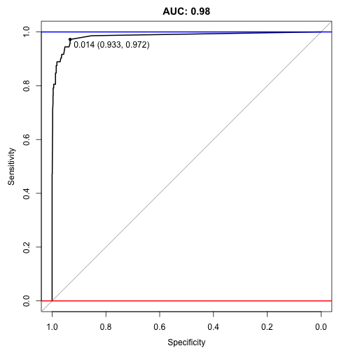
To evaluate the model, we call on package pROC for an auc score and plot:

library(pROC)
auc <- roc(testSplit$target, pred)
print(auc)

## Data: pred in 1509 controls (testSplit$target 0) < 72 cases (testSplit$target 1).
## Area under the curve: 0.985

plot(auc, ylim=c(0,1), print.thres=TRUE, main=paste('AUC:',round(auc$auc[[1]],2)))
abline(h=1,col='blue',lwd=2)
abline(h=0,col='red',lwd=2)

An auc score of 0.98 is great (remember it ranges on a scale between 0.5 and 1, where 0.5 is random and 1 is perfect). It is hard to imagine that SMOTE can improve on this, but…

Let’s SMOTE

Let’s create extra positive observations using SMOTE. We set perc.over = 100 to double the quantity of positive cases, and set perc.under=200 to keep half of what was created as negative cases.

library(DMwR)
trainSplit$target <- as.factor(trainSplit$target)
trainSplit <- SMOTE(target ~ ., trainSplit, perc.over = 100, perc.under=200)
trainSplit$target <- as.numeric(trainSplit$target)

We can check the outcome balance with prop.table and confirm that we equalized the data set between positive and negative cases of hyperthyroidism.

prop.table(table(trainSplit$target))

##   1   2 
## 0.5 0.5

We then train using the SMOTE‘d training set and predict using the same testing set as used before on the non-SMOTE‘d training set to ensure we’re comparing apples-to-apples:

tbmodel <- train(target ~ ., data = trainSplit, method = "treebag",
                 trControl = ctrl)
 
predictors <- names(trainSplit)[names(trainSplit) != 'target']
pred <- predict(tbmodel$finalModel, testSplit[,predictors])

auc <- roc(testSplit$target, pred)
print(auc)

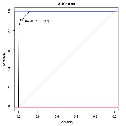
## Data: pred in 1509 controls (testSplit$target 0) < 72 cases (testSplit$target 1).
## Area under the curve: 0.991

Wow 0.991, it managed to better the old auc score of 0.985!

plot(auc, ylim=c(0,1), print.thres=TRUE, main=paste('AUC:',round(auc$auc[[1]],2)))
abline(h=1,col='blue',lwd=2)
abline(h=0,col='red',lwd=2)

Conclusion

Not bad - we ended up reducing the overall size and getting a better score. SMOTE works great in some situation and not-so-great in others. This definitely requires some trial-and-error but the concept is very promising when stuck with extremely skewed and, therefore, overly sensitive data.

Find the full source code and video on ViralML.com