

About Manuel Amunategui
Data scientist with over 20-years experience in the tech industry, MAs in Predictive Analytics and
International Administration, co-author of Monetizing Machine Learning and VP of Data Science at SpringML.
From consulting in machine learning, healthcare modeling, 6 years on Wall Street in the financial industry, and 4 years at Microsoft, I feel like I’ve seen it all. And this has opened my eyes to the huge gap in educational material on applied data science. Like I say:
It just ain’t real 'til it reaches your customer’s plate
I am a startup advisor and available for speaking engagements with companies and schools on topics around building and motivating data science teams, and all things applied machine learning.
Reach me at amunategui@gmail.com


|

Predict Stock-Market Behavior using Markov Chains and R
Practical walkthroughs on machine learning, data exploration and finding insight.

Resources
A
Markov
Chain offers a probabilistic approach in predicting the likelihood
of an event based on previous behavior
(learn
more about Markov Chains here and here).
Past Performance is no Guarantee of Future Results
If you want to experiment whether the stock market is influence by previous market events, then a Markov model is a perfect experimental tool.
We’ll be using Pranab Ghosh’s methodology described in Customer Conversion Prediction with Markov Chain Classifier. Even though he applies it to customer conversion and I apply it to the stock market, the point is that it doesn’t matter where it comes from as long as you can collect enough sequences, even of varying lengths, to find patterns in past behavior.
Some notes: this is just my interpretation using the R language as Pranab uses pseudo code along with a Github repository with Java examples. I hope a am at least capturing his high-level vision as I did take plenty of low-level programming liberties. And, for my fine print, this is only for entertainment and shouldn’t be construed as financial nor trading advice.
Cataloging Patterns Using S&P 500 Market Data
In its raw form, 10 years of S&P 500 index data represents only one sequence of many events leading to the last quoted price. In order to get more sequences and, more importantly, get a better understanding of the market’s behavior, we need to break up the data into many samples of sequences leading to different price patterns. This way we can build a fairly rich catalog of market behaviors and attempt to match them with future patterns to predict future outcomes. For example, below are three sets of consecutive S&P 500 price closes. They represent different periods and contain varying amounts of prices. Think of each of these sequences as a pattern leading to a final price expression. Let’s look at some examples:
2012-10-18 to 2012-11-21
1417.26 –> 1428.39 –> 1394.53 –> 1377.51 –> Next Day Volume Up
2016-08-12 to 2016-08-22
2184.05 –> 2190.15 –> 2178.15 –> 2182.22 –> 2187.02 –> Next Day Volume Up
2014-04-04 to 2014-04-10
1865.09 –> 1845.04 –> Next Day Volume Down
Take the last example, imagine that past three days of the current market match historical behaviors of day 1, 2 and 3. You now have a pattern that matches current market conditions and can use the future price (day 4) as an indicator for tomorrow’s market direction (i.e. market going down). This obviously isn’t using any of Markov’s ideas and is just predicting future behavior on the basis of an up-down-up market pattern.
If you collect thousands and thousands of these sequences, you can build a rich catalog of S&P 500 market behavior. We won’t just compare the closing prices, we’ll also compare the day’s open versus the day’s close, the previous day’s high to the current high, the previous day’s low to the current low, the previous day’s volume to the current one, etc (this will become clearer as we work through the code).
Binning Values Into 3 Buckets
An important twist in Pranab Ghosh’s approach is to simplify each event within a sequence into a single feature. He splits the value into 3 groups - Low, Medium, High. The simplification of the event into three bins will facilitate the subsequent matching between other sequence events and, hopefully, capture the story so it can be used to predict future behavior.
To better generalize stock market data, for example, we can collect the percent difference between one day’s price and the previous day’s. Once we have collected all of them, we can bin them into three groups of equal frequency using the InfoTheo package. The small group is assigned ‘L’, the medium group, ‘M’ and the large, ‘H’.
Here are 6 percentage differences between one close and the previous one:
-0.00061281019 -0.00285190466 0.00266118835 0.00232492640 0.00530862595 0.00512213970
Using equal-frequency binning we can translate the above numbers into:
"M" "L" "M" "M" "H" "H"
Combining Event Features into a Single Event Feature
You then paste all the features for a particular event into a single feature. If we are looking at the percentage difference between closes, opens, highs, lows, we’ll end up with a feature containing four letters. Each representing the bin for that particular feature:
"MLHL"
Then we string all the feature events for the sequence and end up with something like this along with the observed outcome:
"HMLL" "MHHL" "LLLH" "HMMM" "HHHL" "HHHH" --> Volume Up
Creating Two Markov Chains, One for Days with Volume Jumps, and another for Volume Drops
Another twist in Pranab Ghosh’s approach is to separate sequences of events into separate data sets based on the outcome. As we are predicting volume changes, one data set will contain sequences of volume increases and another, decreases. This enables each data set to offer a probability of a directional volume move and the largest probability, wins.
Hi there, this is Manuel Amunategui- if you're enjoying the content, find more at ViralML.com
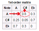
First-Order Transition Matrix
A
transition
matrix is the probability matrix from the Markov Chain. In its
simplest form, you read it by choosing the current event on the y axis
and look for the probability of the next event off the x axis. In the
below image from
Wikipedia,
you see that the highest probability for the next note after A is
C#.
In our case, we will analyze each event pair in a sequence and catalog the market behavior. We then tally all the matching moves and create two data sets for volume action, one for up moves and another for down moves. New stock market events are then broken down into sequential pairs and tallied for both positive and negative outcomes - biggest moves win (there is a little more to this in the code, but that’s it in a nutshell).
Predicting Stock Market Behavior
And now for the final piece you’ve all waited for - let’s turn this thing on and see how well it predicts stock market behavior.
#install.packages('quantmod)
library(quantmod)
#install.packages('dplyr)
library(dplyr)
#install.packages('infotheo)
library(infotheo)
#install.packages('caret')
library(caret)

# get market data
getSymbols(c("^GSPC"))
head(GSPC)
tail(GSPC)
plot(GSPC$GSPC.Volume)

# transfer market data to a simple data frame
GSPC <- data.frame(GSPC)

# extract the date row name into a date column
GSPC$Close.Date <- row.names(GSPC)

# take random sets of sequential rows
new_set <- c()
for (row_set in seq(10000)) {
     row_quant <- sample(10:30, 1)
     print(row_quant)
     row_start <- sample(1:(nrow(GSPC) - row_quant), 1)
     market_subset <- GSPC[row_start:(row_start + row_quant),]
     market_subset <- dplyr::mutate(market_subset,
                                    Close_Date = max(market_subset$Close.Date),
                                    Close_Gap=(GSPC.Close - lag(GSPC.Close))/lag(GSPC.Close) ,
                                    High_Gap=(GSPC.High - lag(GSPC.High))/lag(GSPC.High) ,
                                    Low_Gap=(GSPC.Low - lag(GSPC.Low))/lag(GSPC.Low),
                                    Volume_Gap=(GSPC.Volume - lag(GSPC.Volume))/lag(GSPC.Volume),
                                    Daily_Change=(GSPC.Close - GSPC.Open)/GSPC.Open,
                                    Outcome_Next_Day_Direction= (lead(GSPC.Volume)-GSPC.Volume)) %>%
          dplyr::select(-GSPC.Open, -GSPC.High, -GSPC.Low, -GSPC.Close, -GSPC.Volume, -GSPC.Adjusted, -Close.Date) %>%
          na.omit
     market_subset$Sequence_ID <- row_set
     new_set <- rbind(new_set, market_subset)
}

dim(new_set)

# create sequences
# simplify the data by binning values into three groups

# Close_Gap
range(new_set$Close_Gap)
data_dicretized <- discretize(new_set$Close_Gap, disc="equalfreq", nbins=3)
new_set$Close_Gap <- data_dicretized$X
new_set$Close_Gap_LMH <- ifelse(new_set$Close_Gap == 1, 'L',
                                ifelse(new_set$Close_Gap ==2, 'M','H'))


# Volume_Gap
range(new_set$Volume_Gap)
data_dicretized <- discretize(new_set$Volume_Gap, disc="equalfreq", nbins=3)
new_set$Volume_Gap <- data_dicretized$X
new_set$Volume_Gap_LMH <- ifelse(new_set$Volume_Gap == 1, 'L',
                                 ifelse(new_set$Volume_Gap ==2, 'M','H'))

# Daily_Change
range(new_set$Daily_Change)
data_dicretized <- discretize(new_set$Daily_Change, disc="equalfreq", nbins=3)
new_set$Daily_Change <- data_dicretized$X
new_set$Daily_Change_LMH <- ifelse(new_set$Daily_Change == 1, 'L',
                                   ifelse(new_set$Daily_Change ==2, 'M','H'))

# new set
new_set <- new_set[,c("Sequence_ID", "Close_Date", "Close_Gap_LMH", "Volume_Gap_LMH", "Daily_Change_LMH", "Outcome_Next_Day_Direction")]

new_set$Event_Pattern <- paste0(new_set$Close_Gap_LMH,
                                new_set$Volume_Gap_LMH,
                                new_set$Daily_Change_LMH)

# reduce set
compressed_set <- dplyr::group_by(new_set, Sequence_ID, Close_Date) %>%
     dplyr::summarize(Event_Pattern = paste(Event_Pattern, collapse = ",")) %>%
     data.frame
compressed_set <- merge(x=compressed_set,y=dplyr::select(new_set, Sequence_ID, Outcome_Next_Day_Direction) %>%
                             dplyr::group_by(Sequence_ID) %>%
                             dplyr::slice(n()) %>%
                             dplyr::distinct(Sequence_ID), by='Sequence_ID')

# if you have issues with the above dplyr line, try a workaround from reader - Dysregulation, thanks!
# compressed_set <- merge(x=compressed_set,y=new_set[,c(1,6)], by="Sequence_ID")

# use last x days of data for validation
library(dplyr)
compressed_set_validation <- dplyr::filter(compressed_set, Close_Date >= Sys.Date()-90)
dim(compressed_set_validation)
compressed_set <- dplyr::filter(compressed_set, Close_Date < Sys.Date()-90)
dim(compressed_set)

compressed_set <- dplyr::select(compressed_set, -Close_Date)
compressed_set_validation <- dplyr::select(compressed_set_validation, -Close_Date)

# only keep big moves
summary(compressed_set$Outcome_Next_Day_Direction)
compressed_set <- compressed_set[abs(compressed_set$Outcome_Next_Day_Direction) > 5260500,]
compressed_set$Outcome_Next_Day_Direction <- ifelse(compressed_set$Outcome_Next_Day_Direction > 0, 1, 0)
summary(compressed_set$Outcome_Next_Day_Direction)
dim(compressed_set)
compressed_set_validation$Outcome_Next_Day_Direction <- ifelse(compressed_set_validation$Outcome_Next_Day_Direction > 0, 1, 0)

# create two data sets - won/not won
compressed_set_pos <- dplyr::filter(compressed_set, Outcome_Next_Day_Direction==1) %>% dplyr::select(-Outcome_Next_Day_Direction)
dim(compressed_set_pos)
compressed_set_neg <- dplyr::filter(compressed_set, Outcome_Next_Day_Direction==0) %>% dplyr::select(-Outcome_Next_Day_Direction)
dim(compressed_set_neg)

# build the markov transition grid
build_transition_grid <- function(compressed_grid, unique_patterns) {
     grids <- c()
     for (from_event in unique_patterns) {
          print(from_event)

          # how many times
          for (to_event in unique_patterns) {
               pattern <- paste0(from_event, ',', to_event)
               IDs_matches <- compressed_grid[grep(pattern, compressed_grid$Event_Pattern),]
               if (nrow(IDs_matches) > 0) {
                    Event_Pattern <- paste0(IDs_matches$Event_Pattern, collapse = ',', sep='~~')
                    found <- gregexpr(pattern = pattern, text = Event_Pattern)[[1]]
                    grid <- c(pattern,  length(found))
               } else {
                    grid <- c(pattern,  0)
               }
               grids <- rbind(grids, grid)
          }
     }

     # create to/from grid
     grid_Df <- data.frame(pairs=grids[,1], counts=grids[,2])
     grid_Df$x <- sapply(strsplit(as.character(grid_Df$pairs), ","), `[`, 1)
     grid_Df$y <- sapply(strsplit(as.character(grid_Df$pairs), ","), `[`, 2)
     head(grids)

     all_events_count <- length(unique_patterns)
     transition_matrix = t(matrix(as.numeric(as.character(grid_Df$counts)), ncol=all_events_count, nrow=all_events_count))
     transition_dataframe <- data.frame(transition_matrix)
     names(transition_dataframe) <- unique_patterns
     row.names(transition_dataframe) <- unique_patterns
     head(transition_dataframe)

     # replace all NaN with zeros
     transition_dataframe[is.na(transition_dataframe)] = 0
     # transition_dataframe <- opp_matrix
     transition_dataframe <- transition_dataframe/rowSums(transition_dataframe)
     return (transition_dataframe)
}
unique_patterns <- unique(strsplit(x = paste0(compressed_set$Event_Pattern, collapse = ','), split = ',')[[1]])

grid_pos <- build_transition_grid(compressed_set_pos, unique_patterns)
grid_neg <- build_transition_grid(compressed_set_neg, unique_patterns)

# predict on out of sample data
actual = c()
predicted = c()
for (event_id in seq(nrow(compressed_set_validation))) {
     patterns <- strsplit(x = paste0(compressed_set_validation$Event_Pattern[event_id], collapse = ','), split = ',')[[1]]
     pos <- c()
     neg <- c()
     log_odds <- c()
     for (id in seq(length(patterns)-1)) {

          # logOdds = log(tp(i,j) / tn(i,j)
          log_value <- log(grid_pos[patterns[id],patterns[id+1]] / grid_neg[patterns[id],patterns[id+1]])
          if (is.na(log_value) || (length(log_value)==0) || (is.nan(log(grid_pos[patterns[id],patterns[id+1]] / grid_neg[patterns[id],patterns[id+1]]))==TRUE)) {
               log_value <- 0.0
          } else if (log_value == -Inf) {
               log_value <- log(0.00001 / grid_neg[patterns[id],patterns[id+1]])
          } else if (log_value == Inf) {
               log_value <- log(grid_pos[patterns[id],patterns[id+1]] / 0.00001)

          }
          log_odds <- c(log_odds, log_value)

          pos <- c(pos, grid_pos[patterns[id],patterns[id+1]])
          neg <- c(neg, grid_neg[patterns[id],patterns[id+1]])
     }
     print(paste('outcome:', compressed_set_validation$Outcome_Next_Day_Direction[event_id]))
     print(sum(pos)/sum(neg))
     print(sum(log_odds))

     actual <- c(actual, compressed_set_validation$Outcome_Next_Day_Direction[event_id])
     predicted <- c(predicted, sum(log_odds))

}

  result <- confusionMatrix(ifelse(predicted>0,1,0), actual)
result
A 55% accuracy may not sound like much, but in the world of predicting stock market behavior, anything over a flip-of-a-coin is potentially intesesting.
 Confusion Matrix and Statistics

           Reference
 Prediction   0   1
          0  83  36
          1 110  98

                Accuracy : 0.5535
                  95% CI : (0.4978, 0.6082)
     No Information Rate : 0.5902
     P-Value [Acc > NIR] : 0.9196

                   Kappa : 0.1488
  Mcnemar's Test P-Value : 1.527e-09

             Sensitivity : 0.4301
             Specificity : 0.7313
          Pos Pred Value : 0.6975
          Neg Pred Value : 0.4712
              Prevalence : 0.5902
          Detection Rate : 0.2538
    Detection Prevalence : 0.3639
       Balanced Accuracy : 0.5807

        'Positive' Class : 0
What To Try Next?
You dial up or down the complexity of the pattern, predict others things than volume changes, add more or less sequences, using more bins, etc. Sky’s the limit…
Thanks Lucas A. for the Markov-Dollar-Chains artwork!
Manuel Amunategui - Follow me on Twitter: @amunategui