

About Manuel Amunategui
Data scientist with over 20-years experience in the tech industry, MAs in Predictive Analytics and
International Administration, co-author of Monetizing Machine Learning and VP of Data Science at SpringML.
From consulting in machine learning, healthcare modeling, 6 years on Wall Street in the financial industry, and 4 years at Microsoft, I feel like I’ve seen it all. And this has opened my eyes to the huge gap in educational material on applied data science. Like I say:
It just ain’t real 'til it reaches your customer’s plate
I am a startup advisor and available for speaking engagements with companies and schools on topics around building and motivating data science teams, and all things applied machine learning.
Reach me at amunategui@gmail.com


|

}
Using Correlations To Understand Your Data
Practical walkthroughs on machine learning, data exploration and finding insight.
Resources
Packages Used in this Walkthrough
- {RCurl} - downloads https data
- {psych} - correlation matrix plotting
- {caret} - dummyVars function
A great way to explore new data is to use a pairwise correlation matrix. This will measure the correlation between every combination of your variables. It doesn’t really matter if you have an outcome (or response) variable at this point, it will compare everything against everything else.
For those not familiar with the correlation coefficient, it is simply a measure of similarity between two vectors of numbers. The measure value can range between 1 and -1, where 1 is perfectly correlated, -1 is perfectly inversly correlated, and 0 is not correlated at all:
print(cor(1:5,1:5))
## 1
print(cor(1:5,5:1))
## -1
print(cor(1:5,c(1,2,3,4,4)))
## 0.9701425
To help us understand this process, let’s download the adult.data set from the UCI Machine Learning Repository. The data is from the 1994 Census and attempts to predict those with income under $50,000 a year:
library(RCurl) # download https data
urlfile <- 'https://archive.ics.uci.edu/ml/machine-learning-databases/adult/adult.data'
x <- getURL(urlfile, ssl.verifypeer = FALSE)
adults <- read.csv(textConnection(x), header=F)

# if the above getURL command fails, try this:
# adults <-read.csv('https://archive.ics.uci.edu/ml/machine-learning-databases/adult/adult.data', header=F)
We fill in the missing headers for the UCI set and cast the outcome variable Income to a binary format of 1 and 0 (here I am reversing the orginal order, if it is under $50k, it is 0, and above, 1; this will make the final correlation-matrix plot easier to understand):
names(adults)=c('Age','Workclass','FinalWeight','Education','EducationNumber',
                'MaritalStatus','Occupation','Relationship','Race',
                'Sex','CapitalGain','CapitalLoss','HoursWeek',
                'NativeCountry','Income')

adults$Income <- ifelse(adults$Income==' <=50K',0,1)
We load the caret package to dummify (see my other walkthrough) all factor variables as the cor function only accepts numerical values:
dmy <- dummyVars(" ~ .", data = adults)
adultsTrsf <- data.frame(predict(dmy, newdata = adults))
We borrow two very useful functions from Stephen Turner: cor.prob and flattenSquareMatrix. cor.prob will create a correlation matrix along with p-values and flattenSquareMatrix will flatten all the combinations from the square matrix into a data frame of 4 columns made up of row names, column names, the correlation value and the p-value:
corMasterList <- flattenSquareMatrix (cor.prob(adultsTrsf))
print(head(corMasterList,10))
##                         i                       j       cor         p
## 1                     age            workclass...  0.042627 1.421e-14
## 2                     age  workclass..Federal.gov  0.051227 0.000e+00
## 3            workclass...  workclass..Federal.gov -0.042606 1.454e-14
## 4                     age    workclass..Local.gov  0.060901 0.000e+00
## 5            workclass...    workclass..Local.gov -0.064070 0.000e+00
## 6  workclass..Federal.gov    workclass..Local.gov -0.045682 2.220e-16
## 7                     age workclass..Never.worked -0.019362 4.759e-04
## 8            workclass... workclass..Never.worked -0.003585 5.178e-01
## 9  workclass..Federal.gov workclass..Never.worked -0.002556 6.447e-01
## 10   workclass..Local.gov workclass..Never.worked -0.003843 4.880e-01
This final format allows you to easily order the pairs however you want - for example, by those with the highest absolute correlation value:
corList <- corMasterList[order(-abs(corMasterList$cor)),]
print(head(corList,10))
##                                      i                            j        cor p
## 1953                       sex..Female                    sex..Male -1.0000000 0
## 597                       workclass...                occupation...  0.9979854 0
## 1256 maritalStatus..Married.civ.spouse        relationship..Husband  0.8932103 0
## 1829                       race..Black                  race..White -0.7887475 0
## 527  maritalStatus..Married.civ.spouse maritalStatus..Never.married -0.6448661 0
## 1881             relationship..Husband                  sex..Female -0.5801353 0
## 1942             relationship..Husband                    sex..Male  0.5801353 0
## 1258      maritalStatus..Never.married        relationship..Husband -0.5767295 0
## 1306 maritalStatus..Married.civ.spouse  relationship..Not.in.family -0.5375883 0
## 497                                age maritalStatus..Never.married -0.5343590 0
The top correlated pair (sex..Female and sex.Male), as seen above, won’t be of much use as they are the only two levels of the same factor. We need to process this a little further to be of practical use. We create a single vector of variable names by filtering those with an absolute correlation of 0.2 or higher against the outcome variable of Income:
selectedSub <- subset(corList, (abs(cor) > 0.2 & j == 'Income'))
print(selectedSub)
                                     i      j        cor p
## 5811      MaritalStatus..Never.married Income -0.3184403 0
## 5832           Relationship..Own.child Income -0.2285320 0
## 5840                       Sex..Female Income -0.2159802 0
## 5818       Occupation..Exec.managerial Income  0.2148613 0
## 5841                         Sex..Male Income  0.2159802 0
## 5842                       CapitalGain Income  0.2233288 0
## 5844                         HoursWeek Income  0.2296891 0
## 5779                               Age Income  0.2340371 0
## 5806                  Education.Number Income  0.3351540 0
## 5829             Relationship..Husband Income  0.4010353 0
## 5809 MaritalStatus..Married.civ.spouse Income  0.4446962 0
We save the most correlated features to the bestSub variable:
bestSub <- as.character(selectedSub$i)
Hi there, this is Manuel Amunategui- if you're enjoying the content, find more at ViralML.com
Finally we plot the highly correlated pairs using the {psych} package’s pair.panels plot (this can also be done on the original data as pair.panels can handle factor and character variables):
library(psych)
pairs.panels(adultsTrsf[c(bestSub, 'Income')])
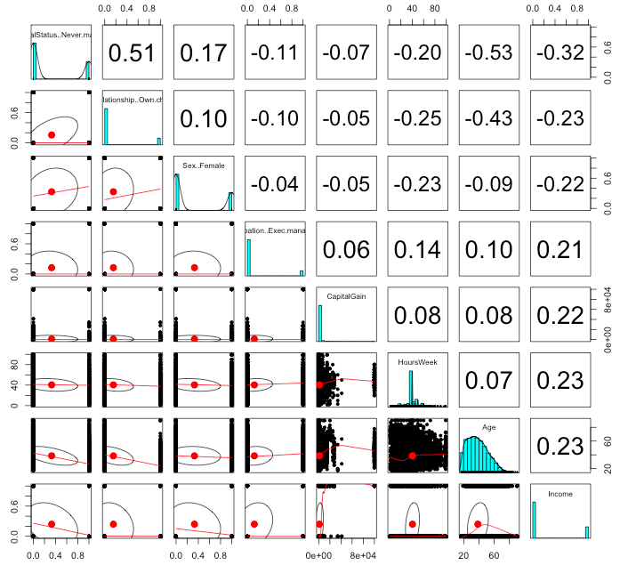
The pairs plot, and in particular the last Income column, tell us a lot about our data set. Being never married is the most negatively correlated with income over $50,000/year and Hours Worked and Age are the most postively correlated.
Things to keep in mind
Full source code (also on GitHub):
library(RCurl) # download https data
urlfile <- 'https://archive.ics.uci.edu/ml/machine-learning-databases/adult/adult.data'
x <- getURL(urlfile, ssl.verifypeer = FALSE)
adults <- read.csv(textConnection(x), header=F)

# if the above getURL command fails, try this:
# adults <-read.csv('https://archive.ics.uci.edu/ml/machine-learning-databases/adult/adult.data', header=F)

names(adults)=c('Age','Workclass','FinalWeight','Education','EducationNumber',
                'MaritalStatus','Occupation','Relationship','Race',
                'Sex','CapitalGain','CapitalLoss','HoursWeek',
                'NativeCountry','Income')

adults$Income <- ifelse(adults$Income==' <=50K',0,1)

library(caret)
dmy <- dummyVars(" ~ .", data = adults)
adultsTrsf <- data.frame(predict(dmy, newdata = adults))

## Correlation matrix with p-values. See http://goo.gl/nahmV for documentation of this function
cor.prob <- function (X, dfr = nrow(X) - 2) {
        R <- cor(X, use="pairwise.complete.obs")
        above <- row(R) < col(R)
        r2 <- R[above]^2
        Fstat <- r2 * dfr/(1 - r2)
        R[above] <- 1 - pf(Fstat, 1, dfr)
        R[row(R) == col(R)] <- NA
        R
}

## Use this to dump the cor.prob output to a 4 column matrix
## with row/column indices, correlation, and p-value.
## See StackOverflow question: http://goo.gl/fCUcQ
flattenSquareMatrix <- function(m) {
        if( (class(m) != "matrix") | (nrow(m) != ncol(m))) stop("Must be a square matrix.")
        if(!identical(rownames(m), colnames(m))) stop("Row and column names must be equal.")
        ut <- upper.tri(m)
        data.frame(i = rownames(m)[row(m)[ut]],
                   j = rownames(m)[col(m)[ut]],
                   cor=t(m)[ut],
                   p=m[ut])
}

corMasterList <- flattenSquareMatrix (cor.prob(adultsTrsf))
print(head(corMasterList,10))

corList <- corMasterList[order(-abs(corMasterList$cor)),]
print(head(corList,10))

corList <- corMasterList[order(corMasterList$cor),]
selectedSub <- subset(corList, (abs(cor) > 0.2 & j == 'Income'))
# to get the best variables from original list:
bestSub <-  sapply(strsplit(as.character(selectedSub$i),'[.]'), "[", 1)
bestSub <- unique(bestSub)

# or use the variables from top selectedSub:
bestSub <- as.character(selectedSub$i)

library(psych)
pairs.panels(adultsTrsf[c(bestSub, 'Income')])
Manuel Amunategui - Follow me on Twitter: @amunategui