

About Manuel Amunategui
Data scientist with over 20-years experience in the tech industry, MAs in Predictive Analytics and
International Administration, co-author of Monetizing Machine Learning and VP of Data Science at SpringML.
From consulting in machine learning, healthcare modeling, 6 years on Wall Street in the financial industry, and 4 years at Microsoft, I feel like I’ve seen it all. And this has opened my eyes to the huge gap in educational material on applied data science. Like I say:
It just ain’t real 'til it reaches your customer’s plate
I am a startup advisor and available for speaking engagements with companies and schools on topics around building and motivating data science teams, and all things applied machine learning.
Reach me at amunategui@gmail.com


|

Using String Distance {stringdist} To Handle Large Text Factors, Cluster Them Into Supersets
Practical walkthroughs on machine learning, data exploration and finding insight.
Resources
Packages Used in this Walkthrough
- {stringdist} - feature selection for ensembles
- {RCurl} - machine learning tools
If you’re wondering whether you’re getting the most out of a text-based, factor variable from a large data set, then you’re not alone. There are so many ways of deconstructing text variables. If every entry is made of repeated text from a small set of possibilities, then dummifying it is the easiest way to proceed. On the other hand, if every entry is unique, then resorting to Natural Language Processing (NLP) may be required. This article tackles the gray area in between, where the data is neither unique nor small, where dummifying won’t work yet NLP may still be avoided.
So that we are on the same page, imagine a data set with 10 million rows with at least one feature/column being a text-based factor. It is not made up of free-text, where every entry is unique, instead, it is made up of repeated text: for example 10,000 possibilities repeated over 10 million rows. This would be hard to dummify, as it will blow up your feature space, and would take forever to group by hand.
What Is One To Do?
- We could encode the text entries as integers or binaries and hope for the best (as it is not ordinal in nature, linear models would suffer but classification models would be OK).
- We could take the top X most popular ones and overwrite the rest as 'other' and dummify the resulting set (I have used that method many times and will write up a post on the subject).
- But a more interesting approach that affords much less loss of information, is grouping them into supersets and the subject of this walkthrough.
Grouping With {stringdist}
Could those 10,000 possibilities mentioned earlier be grouped into a superset representing only a tenth or a fifth of its original size? What is close to impossible to do by hand is trivial with string distance:
...a metric that measures distance ("inverse similarity") between two text strings for approximate string matching or comparison and in fuzzy string searching. (Source: Wikipedia)
The {strndist} package offers ‘Approximate string matching and string distance functions’. It offers many algorithms but the two I found the most interesting for short sets of words are:
...the Jaro–Winkler distance (Winkler, 1990) is a measure of similarity between two strings. The higher the Jaro–Winkler distance for two strings is, the more similar the strings are. The Jaro–Winkler distance metric is designed and best suited for short strings such as person names. The score is normalized such that 0 equates to no similarity and 1 is an exact match. (Source: Wikipedia)
and
...the Levenshtein distance between two words is the minimum number of single-character edits (i.e. insertions, deletions or substitutions) required to change one word into the other. (Source: Wikipedia)
Hi there, this is Manuel Amunategui- if you're enjoying the content, find more at ViralML.com
Let’s Code!
Enough chitchat, let’s download the vehicles data set from Hadley Wickham hosted on Github. It is a big and diverse data set, perfect for our needs:
library(RCurl)
urlfile <-'https://raw.githubusercontent.com/hadley/fueleconomy/master/data-raw/vehicles.csv'
x <- getURL(urlfile, ssl.verifypeer = FALSE)
vehicles <- read.csv(textConnection(x))

# alternative way of getting the data if the above snippet doesn't work:
# urlData <- getURL('https://raw.githubusercontent.com/hadley/fueleconomy/master/data-raw/vehicles.csv')
# vehicles <- read.csv(text = urlData)
We’re going to focus on one single feature in the data set: model. Let’s start with some basic statistics on that feature to understand what we’re dealing with:
nrow(vehicles)
[1] 34631
length(unique(vehicles$model))
[1] 3234
So, we have a data set of over 34,631 vehicles, but model is comprised of only 3,234 unique model names repeated through out all the observations/rows. Let’s look at the first 100 rows so we don’t get overwhelmed with too much the data:
vehicles_small <- vehicles[1:100,]
Out of those 100 observations, model has only 45 unique model names and here is a small sample of what it holds:
length(unique(vehicles_small$model))
[1] 45
head(unique(as.character(vehicles_small$model)))
[1] "Spider Veloce 2000"  "Testarossa"          "Charger"
[4] "B150/B250 Wagon 2WD" "Legacy AWD Turbo"    "Loyale"
Let’s run some basic string distance on this subset by calling the stringdistmatrix function to see how it can help us tame the model variable into smaller supersets. In its simplest form, the function stringdistmatrix only requires a unique set of text values and the method to cluster the data:
stringdistmatrix(a, b, method = c("osa", "lv", "dl", "hamming", "lcs",
        "qgram", "cosine", "jaccard", "jw", useBytes = FALSE,
        weight = c(d = 1, i = 1, s = 1, t = 1), maxDist = Inf, q = 1, p = 0,
        useNames = FALSE, ncores = 1, cluster = NULL)
We’ll pass it the unique list of models, request the Jaro–Winkler distance algorithm (my favorite for this task), cluster the results into 20 groups with the hclust function and plot the resulting dendrogram:
library(stringdist)
uniquemodels <- unique(as.character(vehicles_small$model))
distancemodels <- stringdistmatrix(uniquemodels,uniquemodels,method = "jw")
rownames(distancemodels) <- uniquemodels
hc <- hclust(as.dist(distancemodels))
plot(hc)
rect.hclust(hc,k=20)
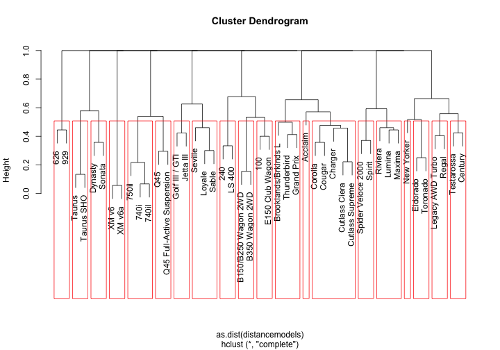
stringdistmatrix works in tandem with hclust, one creates the model, the other enforces the clusters. Our algorithm created a Wagon and Taurus group along with some number groups. So far it isn’t extremely impressive as its only using a small subset of data - wait till we open things up!
We now look at a bigger subset of the vehicles data set. Let’s pull the first 2000 observations:
vehicles_small <- vehicles[1:2000,]
length(unique(vehicles_small$model))
[1] 481
Out of those 2000 observations, we have 481 unique model names. Let’s ask stringdistmatrix to group those into 200 groups:
uniquemodels <- unique(as.character(vehicles_small$model))
distancemodels <- stringdistmatrix(uniquemodels,uniquemodels,method = "jw")
rownames(distancemodels) <- uniquemodels
hc <- hclust(as.dist(distancemodels))
dfClust <- data.frame(uniquemodels, cutree(hc, k=200))
names(dfClust) <- c('modelname','cluster')
Let’s visualize the quantities of models in each group created by the Jaro–Winkler distance algorithm:
plot(table(dfClust$cluster))

print(paste('Average number of models per cluster:', mean(table(dfClust$cluster))))
## [1] "Average number of models per cluster: 2.405"
The largest cluster contains over 10 models but the average is 2.4 models per cluster. Now, lets look at the top groups and see what the algorithm did (don’t sweat this code, it simply orders the data by cluster size):
t <- table(dfClust$cluster)
t <- cbind(t,t/length(dfClust$cluster))
t <- t[order(t[,2], decreasing=TRUE),]
p <- data.frame(factorName=rownames(t), binCount=t[,1], percentFound=t[,2])
dfClust <- merge(x=dfClust, y=p, by.x = 'cluster', by.y='factorName', all.x=T)
dfClust <- dfClust[rev(order(dfClust$binCount)),]
names(dfClust) <-  c('cluster','modelname')
head (dfClust[c('cluster','modelname')],50)
##     cluster              modelname
## 192      73       K1500 Pickup 4WD
## 191      73         S10 Pickup 2WD
## 190      73        W250 Pickup 4WD
## 189      73        F150 Pickup 2WD
## 188      73         S10 Pickup 4WD
## 187      73   D100/D150 Pickup 2WD
## 186      73        F250 Pickup 2WD
## 185      73       C1500 Pickup 2WD
## 184      73        F150 Pickup 4WD
## 183      73        D250 Pickup 2WD
## 182      73   W100/W150 Pickup 4WD
## 341     123 Postal Cab Chassis 2WD
## 340     123    S10 Cab Chassis 2WD
## 339     123 Dakota Cab Chassis 2WD
## 338     123        Cab/Chassis 2WD
## 337     123        Cab Chassis 2WD
## 336     123    S15 Cab Chassis 2WD
## 335     123  Truck Cab Chassis 2WD
## 334     123   D250 Cab Chassis 2WD
## 236      84         Yukon 1500 4WD
## 235      84       Suburban C10 2WD
## 234      84            SJ 410V 4WD
## 233      84      Suburban 1500 2WD
## 232      84       Suburban K10 4WD
## 231      84        Yukon K1500 4WD
## 230      84             SJ 410 4WD
## 229      84      Suburban 1500 4WD
## 365     130        900 Convertible
## 364     130       318i Convertible
## 363     130            Convertible
## 362     130    XJS V12 Convertible
## 361     130       E320 Convertible
## 360     130       325i Convertible
## 359     130        XJS Convertible
## 307     107     Sidekick 2Door 2WD
## 306     107   Sidekick Hardtop 2WD
## 305     107     Sidekick 4Door 2WD
## 304     107     Sidekick 2Door 4WD
## 303     107           Sidekick 2WD
## 302     107   Sidekick Hardtop 4WD
## 301     107     Sidekick 4Door 4WD
## 86       36              240 Wagon
## 85       36             E320 Wagon
## 84       36              940 Wagon
## 83       36              850 Wagon
## 82       36              960 Wagon
## 81       36        E150 Club Wagon
## 80       36              100 Wagon
## 13        5       Legacy AWD Turbo
## 12        5           Legacy Wagon
Out of the 200 clusters we requested, cluster 73 is the largest holding 11 models. Clearly, it picked up on the word pickup flanked by two words on either side with the right one being 2WD or 4WD. Cluster 123 looked for Cab Chassis, even picking up a Cab/Chassis in the process. You get the idea and, hopefully, are impressed with how a few lines of code reduced 2000 observations into 200 groups. The exact same process would apply to 20,000 observations or 20 million…
Creating New Variables Through Combining Multiple Features
An offshoot of this process is to create new groups by combining existing features and running the results through stringdistmatrix. Let’s try combining model with trany:
vehicles_small$modelAndTrany <- paste0(as.character(vehicles_small$model)," ",as.character(vehicles_small$trany))
print(length(unique(vehicles_small$modelAndTrany)))
## [1] 808
Our new field has 808 unique values out of our 2000 small_vehicles data frame. Let’s run it through the Jaro–Winkler distance algorithm, request 500 clusters and check out the top groups:
uniquemodels <- unique(as.character(vehicles_small$modelAndTrany))
distancemodels <- stringdistmatrix(uniquemodels,uniquemodels,method = "jw")
rownames(distancemodels) <- uniquemodels
hc <- hclust(as.dist(distancemodels))
dfClust <- data.frame(uniquemodels, cutree(hc, k=500))
names(dfClust) <- c('modelname','cluster')
t <- table(dfClust$cluster)
t <- cbind(t,t/length(dfClust$cluster))
t <- t[order(t[,2], decreasing=TRUE),]
p <- data.frame(factorName=rownames(t), binCount=t[,1], percentFound=t[,2])
dfClust <- merge(x=dfClust, y=p, by.x = 'cluster', by.y='factorName', all.x=T)
dfClust <- dfClust[rev(order(dfClust$binCount)),]
names(dfClust) <-  c('cluster','modelname')
head (dfClust[c('cluster','modelname')],50)
##     cluster                           modelname
## 38       16                 960 Automatic 4-spd
## 37       16                  90 Automatic 4-spd
## 36       16                 940 Automatic 4-spd
## 35       16                 900 Automatic 4-spd
## 34       16                E500 Automatic 4-spd
## 33       16                 100 Automatic 4-spd
## 32       16                9000 Automatic 4-spd
## 31       16                 850 Automatic 4-spd
## 27       14                 G20 Automatic 4-spd
## 26       14                 240 Automatic 4-spd
## 25       14                S420 Automatic 4-spd
## 24       14               240SX Automatic 4-spd
## 23       14                C280 Automatic 4-spd
## 22       14                C220 Automatic 4-spd
## 21       14                E420 Automatic 4-spd
## 221     120           960 Wagon Automatic 4-spd
## 220     120          E320 Wagon Automatic 4-spd
## 219     120           850 Wagon Automatic 4-spd
## 218     120           240 Wagon Automatic 4-spd
## 217     120           100 Wagon Automatic 4-spd
## 216     120           940 Wagon Automatic 4-spd
## 185      99                     SW Manual 5-spd
## 184      99                     S4 Manual 5-spd
## 183      99                     S6 Manual 5-spd
## 182      99                    NSX Manual 5-spd
## 181      99                     SL Manual 5-spd
## 180      99                     SC Manual 5-spd
## 248     129    Ram 1500 Pickup 4WD Manual 5-spd
## 247     129    Ram 2500 Pickup 2WD Manual 5-spd
## 246     129    Ram 2500 Pickup 4WD Manual 5-spd
## 245     129    Ram 1500 Pickup 2WD Manual 5-spd
## 244     129      Ram 50 Pickup 2WD Manual 5-spd
## 243     128 Ram 1500 Pickup 2WD Automatic 4-spd
## 242     128 Ram 2500 Pickup 4WD Automatic 4-spd
## 241     128   Ram 50 Pickup 2WD Automatic 4-spd
## 240     128 Ram 1500 Pickup 4WD Automatic 4-spd
## 239     128 Ram 2500 Pickup 2WD Automatic 4-spd
## 177      97                 NSX Automatic 4-spd
## 176      97                  SC Automatic 4-spd
## 175      97                 SVX Automatic 4-spd
## 174      97                  SW Automatic 4-spd
## 173      97                  SL Automatic 4-spd
## 154      83               SL600 Automatic 4-spd
## 153      83              500SEL Automatic 4-spd
## 152      83               SL500 Automatic 4-spd
## 151      83              400SEL Automatic 4-spd
## 150      83               500SL Automatic 4-spd
## 47       18                540i Automatic 5-spd
## 46       18               840ci Automatic 5-spd
## 45       18               740il Automatic 5-spd
Conclusion
stringdistmatrix is a very flexible function with many tunable features. The cluster size, the algorithm, the concatenation of text with text and/or numbers create numerous and mind-boggling possibilities. Even with all these settings it is still so much easier than creating supersets by hand! String distance matching is case sensitive so you may get better groups if you force all text to once case. Have fun with this…
Full source code (also on GitHub):
# get the Hadley Wickham's vehicles data set
library(RCurl)
urlfile <-'https://raw.githubusercontent.com/hadley/fueleconomy/master/data-raw/vehicles.csv'
x <- getURL(urlfile, ssl.verifypeer = FALSE)
vehicles <- read.csv(textConnection(x))

# size the data
nrow(vehicles)
length(unique(vehicles$model))

# get a small sample for starters
vehicles_small <- vehicles[1:100,]
length(unique(vehicles_small$model))
head(unique(as.character(vehicles_small$model)))

# call the stringdistmatrix function and request 20 groups
library(stringdist)
uniquemodels <- unique(as.character(vehicles_small$model))
distancemodels <- stringdistmatrix(uniquemodels,uniquemodels,method = "jw")
rownames(distancemodels) <- uniquemodels
hc <- hclust(as.dist(distancemodels))

# visualize the dendrogram
plot(hc)
rect.hclust(hc,k=20)

# get a bigger sample
vehicles_small <- vehicles[1:2000,]
length(unique(vehicles_small$model))

# run the stringdistmatrix function and request 200 groups
uniquemodels <- unique(as.character(vehicles_small$model))
distancemodels <- stringdistmatrix(uniquemodels,uniquemodels,method = "jw")
rownames(distancemodels) <- uniquemodels
hc <- hclust(as.dist(distancemodels))
dfClust <- data.frame(uniquemodels, cutree(hc, k=200))
names(dfClust) <- c('modelname','cluster')

# visualize the groupings
plot(table(dfClust$cluster))
print(paste('Average number of models per cluster:', mean(table(dfClust$cluster))))

# lets look at the top groups and see what the algorithm did:
t <- table(dfClust$cluster)
t <- cbind(t,t/length(dfClust$cluster))
t <- t[order(t[,2], decreasing=TRUE),]
p <- data.frame(factorName=rownames(t), binCount=t[,1], percentFound=t[,2])
dfClust <- merge(x=dfClust, y=p, by.x = 'cluster', by.y='factorName', all.x=T)
dfClust <- dfClust[rev(order(dfClust$binCount)),]
names(dfClust) <-  c('cluster','modelname')
head (dfClust[c('cluster','modelname')],50)

# try combining fields together
vehicles_small$modelAndTrany <- paste0(as.character(vehicles_small$model)," ",as.character(vehicles_small$trany))
print(length(unique(vehicles_small$modelAndTrany)))

uniquemodels <- unique(as.character(vehicles_small$modelAndTrany))
distancemodels <- stringdistmatrix(uniquemodels,uniquemodels,method = "jw")
rownames(distancemodels) <- uniquemodels
hc <- hclust(as.dist(distancemodels))
dfClust <- data.frame(uniquemodels, cutree(hc, k=500))
names(dfClust) <- c('modelname','cluster')
t <- table(dfClust$cluster)
t <- cbind(t,t/length(dfClust$cluster))
t <- t[order(t[,2], decreasing=TRUE),]
p <- data.frame(factorName=rownames(t), binCount=t[,1], percentFound=t[,2])
dfClust <- merge(x=dfClust, y=p, by.x = 'cluster', by.y='factorName', all.x=T)
dfClust <- dfClust[rev(order(dfClust$binCount)),]
names(dfClust) <-  c('cluster','modelname')
head (dfClust[c('cluster','modelname')],50)

# build a convenient function to do all of the above
GroupFactorsTogether <- function(objData, variableName, clustersize=200, method='jw') {
        #      osa: Optimal string aligment, (restricted Damerau-Levenshtein distance).
        #      lv: Levenshtein distance (as in R's native adist).
        #      dl: Full Damerau-Levenshtein distance.
        #      hamming: Hamming distance (a and b must have same nr of characters).
        #      lcs: Longest common substring distance.
        #      qgram: q-gram distance.
        #      cosine: cosine distance between q-gram profiles
        #      jaccard: Jaccard distance between q-gram profiles
        #      jw: Jaro, or Jaro-Winker distance.
        #      soundex: Distance based on soundex encoding

        #       stringdistmatrix(a, b, method = c("osa", "lv", "dl", "hamming", "lcs",
        #               "qgram", "cosine", "jaccard", "jw", useBytes = FALSE,
        #               weight = c(d = 1, i = 1, s = 1, t = 1), maxDist = Inf, q = 1, p = 0,
        #               useNames = FALSE, ncores = 1, cluster = NULL)
        #               require(stringdist)

        str <- unique(as.character(objData[,variableName]))
        print(paste('Uniques:',length(str)))

        d <- stringdistmatrix(str,str,method = c(method))

        rownames(d) <- str
        hc <- hclust(as.dist(d))

        dfClust <- data.frame(str, cutree(hc, k=clustersize))

        plot(table(dfClust$'cutree.hc..k...k.'))

        most_populated_clusters <- dfClust[dfClust$'cutree.hc..k...k.' > 5,]
        names(most_populated_clusters) <- c('entry','cluster')

        # sort by most frequent
        t <- table(most_populated_clusters$cluster)
        t <- cbind(t,t/length(most_populated_clusters$cluster))
        t <- t[order(t[,2], decreasing=TRUE),]
        p <- data.frame(factorName=rownames(t), binCount=t[,1], percentFound=t[,2])
        most_populated_clusters <- merge(x=most_populated_clusters, y=p, by.x = 'cluster', by.y='factorName', all.x=T)
        most_populated_clusters <- most_populated_clusters[rev(order(most_populated_clusters$binCount)),]
        names(most_populated_clusters) <-  c('cluster','entry')
        return (most_populated_clusters[c('cluster','entry')])
}
Manuel Amunategui - Follow me on Twitter: @amunategui