

About Manuel Amunategui
Data scientist with over 20-years experience in the tech industry, MAs in Predictive Analytics and
International Administration, co-author of Monetizing Machine Learning and VP of Data Science at SpringML.
From consulting in machine learning, healthcare modeling, 6 years on Wall Street in the financial industry, and 4 years at Microsoft, I feel like I’ve seen it all. And this has opened my eyes to the huge gap in educational material on applied data science. Like I say:
It just ain’t real 'til it reaches your customer’s plate
I am a startup advisor and available for speaking engagements with companies and schools on topics around building and motivating data science teams, and all things applied machine learning.
Reach me at amunategui@gmail.com


|

Mapping The United States Census With {ggmap}
Practical walkthroughs on machine learning, data exploration and finding insight.
Resources
Packages Used in this Walkthrough
- {RCurl} - downloads https data
- {xlsx} - Excel reader
- {zipcode} - US zipcode tools and data
- {ggmap} - map visualization
- {ggplot2} - graphics
If you haven’t played with the ggmap package then you’re in for a treat! It will map your data on any location around the world as long as you give it proper geographical coordinates.
Even though ggmap supports different map providers, I have only used it with Google Maps and that is what I will demonstrate in this article. We’re going to download the median household income for the United States from the 2006 to 2010 census. Normally you would need to download a shape file from the Census.gov site but the University of Michigan’s Institute for Social Research graciously provides an Excel file for the national numbers. The file is limited to the mean and median household numbers for every zip code in the United States.
We’re going to load two packages in order to download the data: RCurl to handle HTTP protocols to download the file directly from the Internet and xlsx to read the Excel file and load the sheet named ‘Median’ into our data.frame:
urlfile <-'http://www.psc.isr.umich.edu/dis/census/Features/tract2zip/MedianZIP-3.xlsx'
destfile <- "census20062010.xlsx"
download.file(urlfile, destfile, mode="wb")
census <- read.xlsx2(destfile, sheetName = "Median")

# NOTE: if you can't download the file automatically, download it manually at:
# 'http://www.psc.isr.umich.edu/dis/census/Features/tract2zip/'
We clean the file by keeping only the zip code and median household income variables and casting the median figures from factor to numbers:
census <- census[c('Zip','Median..')]
names(census) <- c('Zip','Median')
census$Median <- as.character(census$Median)
census$Median <- as.numeric(gsub(',','',census$Median))
print(head(census,5))
##    Zip Median
## 1 1001  56663
## 2 1002  49853
## 3 1003  28462
## 4 1005  75423
## 5 1007  79076
You will notice that the zip codes above only have 4 digits. We leverage another package called zipcode to not only clean our zip codes by removing any ‘+4’ data and padding with zeros where needed, but more importantly, to give us the central latitude and longitude coordinate for our zip codes (this requires downloading the zipcode data file):
data(zipcode)
census$Zip <- clean.zipcodes(census$Zip)
We merge our census data with the zipcode data on zip codes:
census <- merge(census, zipcode, by.x='Zip', by.y='zip')
Finally, we reach the heart of our mapping goal, we download a map of the United States using ggmap. For a more detailed introduction to ggmap, check out this article written by the authors of the package. The get_map function downloads the map as an image. Amongst the available parameters, we opt for zoom level 4 (which works well to cover the US), and request a colored, terrain-type map (versus satellite or black and white, amongst many otherr options):
map<-get_map(location='united states', zoom=4, maptype = "terrain",
             source='google',color='color')
## Map from URL : http://maps.googleapis.com/maps/api/staticmap?center=united+states&zoom=4&size=%20640x640&scale=%202&maptype=terrain&sensor=false
## Google Maps API Terms of Service : http://developers.google.com/maps/terms
## Information from URL : http://maps.googleapis.com/maps/api/geocode/json?address=united+states&sensor=false
## Google Maps API Terms of Service : http://developers.google.com/maps/terms
And ggplot2 that will handle the graphics (based on the grammar of graphics) where we pass our census data with the geographical coordinates:
ggmap(map) + geom_point(
        aes(x=longitude, y=latitude, show_guide = TRUE, colour=Median),
        data=census, alpha=.5, na.rm = T)  +
        scale_color_gradient(low="beige", high="blue")
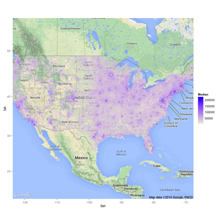
And there you have it, the median household income from 2006 to 2010 mapped onto a Google Map of the US in just a few lines of code! You can play around with the alpha setting to increase or decrease the transparency of the census data on the map.
Hi there, this is Manuel Amunategui- if you're enjoying the content, find more at ViralML.com
Full source code (also on GitHub):
require(RCurl)
require(xlsx)

# NOTE if you can't download the file automatically, download it manually at:
# 'http://www.psc.isr.umich.edu/dis/census/Features/tract2zip/'
urlfile <-'http://www.psc.isr.umich.edu/dis/census/Features/tract2zip/MedianZIP-3.xlsx'
destfile <- "census20062010.xlsx"
download.file(urlfile, destfile, mode="wb")
census <- read.xlsx2(destfile, sheetName = "Median")

# clean up data
census <- census[c('Zip','Median..')]
names(census) <- c('Zip','Median')
census$Median <- as.character(census$Median)
census$Median <- as.numeric(gsub(',','',census$Median))
print(head(census,5))

# get geographical coordinates from zipcode
require(zipcode)
data(zipcode)
census$Zip <- clean.zipcodes(census$Zip)
census <- merge(census, zipcode, by.x='Zip', by.y='zip')

# get a Google map
require(ggmap)
map<-get_map(location='united states', zoom=4, maptype = "terrain",
             source='google',color='color')

# plot it with ggplot2
require("ggplot2")
ggmap(map) + geom_point(
        aes(x=longitude, y=latitude, show_guide = TRUE, colour=Median),
        data=census, alpha=.8, na.rm = T)  +
        scale_color_gradient(low="beige", high="blue")
Manuel Amunategui - Follow me on Twitter: @amunategui