

About Manuel Amunategui
Data scientist with over 20-years experience in the tech industry, MAs in Predictive Analytics and
International Administration, co-author of Monetizing Machine Learning and VP of Data Science at SpringML.
From consulting in machine learning, healthcare modeling, 6 years on Wall Street in the financial industry, and 4 years at Microsoft, I feel like I’ve seen it all. And this has opened my eyes to the huge gap in educational material on applied data science. Like I say:
It just ain’t real 'til it reaches your customer’s plate
I am a startup advisor and available for speaking engagements with companies and schools on topics around building and motivating data science teams, and all things applied machine learning.
Reach me at amunategui@gmail.com


|

Ensemble Feature Selection On Steroids: {fscaret} Package
Practical walkthroughs on machine learning, data exploration and finding insight.
Resources
Packages Used in this Walkthrough
- {fscaret} - feature selection for ensembles
- {caret} - machine learning tools
The fscaret package, as its name implies, is closely related to the caret package. It relies on caret, and its numerous functions, to get its job done.
So what does this package do?
Well, you give it a data set and a list of models and, in return, fscaret will scale and return the importance of each variable for each model and for the ensemble of models. The tool extracts the importance of each variable by using the selected models’ VarImp or similar measuring function. For example, linear models use the absolute value of the t-statistic for each parameter and decision-tree models, total the importance of the individual trees, etc. It returns individual and combined MSEs and RMSEs:
Now, caret is itself a wrapper sitting atop 170 models and offering many machine learning and tuning functions. I will assume you are familiar with caret, but even if you aren’t, fscaret is intuitive enough to provide lots of use on its own as an ensemble variable selection tool (but do get to know caret, you won’t regret it).
To get a full list of all the models available with the fscaret package (which is over a third of the models supported in caret), install and load the fscaret package then type in the following:
library(fscaret)
data(funcRegPred)
print(funcRegPred)
##  [1] "glm"            "glmStepAIC"     "gam"            "gamLoess"
##  [5] "gamSpline"      "rpart"          "rpart2"         "ctree"
##  [9] "ctree2"         "evtree"         "obliqueTree"    "gbm"
## [13] "blackboost"     "bstTree"        "glmboost"       "gamboost"
## [17] "bstLs"          "bstSm"          "rf"             "parRF"
## [21] "cforest"        "Boruta"         "RRFglobal"      "RRF"
## [25] "treebag"        "bag"            "logicBag"       "bagEarth"
## [29] "nodeHarvest"    "partDSA"        "earth"          "gcvEarth"
## [33] "logreg"         "glmnet"         "nnet"           "mlp"
## [37] "mlpWeightDecay" "pcaNNet"        "avNNet"         "rbf"
## [41] "pls"            "kernelpls"      "simpls"         "widekernelpls"
## [45] "spls"           "svmLinear"      "svmRadial"      "svmRadialCost"
## [49] "svmPoly"        "gaussprLinear"  "gaussprRadial"  "gaussprPoly"
## [53] "knn"            "xyf"            "bdk"            "lm"
## [57] "lmStepAIC"      "leapForward"    "leapBackward"   "leapSeq"
## [61] "pcr"            "icr"            "rlm"            "neuralnet"
## [65] "qrf"            "qrnn"           "M5Rules"        "M5"
## [69] "cubist"         "ppr"            "penalized"      "ridge"
## [73] "lars"           "lars2"          "enet"           "lasso"
## [77] "relaxo"         "foba"           "krlsRadial"     "krlsPoly"
## [81] "rvmLinear"      "rvmRadial"      "rvmPoly"        "superpc"
And compare that with the models supported in caret (install and load the caret package):
library(caret)
print(paste('Total models in caret:', length(getModelInfo())))
## [1] "Total models in caret: 169"
# to get full list of supported models type:
# names(getModelInfo())
Even though caret supports a lot more than those 84 models, it should be plenty of fire power to select the best variables possible for your needs. When installing fscaret, it is recommended to install it with all its dependencies:
install.packages("fscaret", dependencies = c("Depends", "Suggests"))
This will speed things up tremendously on subsequent runs but you will have to suffer during the installation process. If I remember correctly, it took me over an hour to get all the models installed (some of the models require user confirmations).
The input data needs to be formatted in a particular way: MISO. (Multiple Ins, Single Out). The output needs be the last column in the data frame. So you can’t have it anywhere else, nor can it predict multiple response columns at once.
As with anything ensemble related, if you’re going to run 50 models in one shot, you better have the computing muscle to do so - there’s no free lunch. Start with a single or small set of models. If you’re going to run a large ensemble of models, fire it up before going to bed and see what you get the next day.
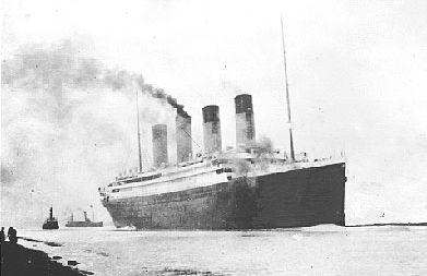
For the demo, we’ll use a Titanic dataset from the University of Colorado Denver. This is a classic data set often seen in online courses and walkthroughs. The outcome is passenger survivorship (i.e. can you predict who will survive based on various features). We drop the passenger names as they are all unique but keep the passenger titles. We also impute the missing ‘Age’ variables with the mean:
titanicDF <- read.csv('http://math.ucdenver.edu/RTutorial/titanic.txt',sep='\t')
titanicDF$Title <- ifelse(grepl('Mr ',titanicDF$Name),'Mr',ifelse(grepl('Mrs ',titanicDF$Name),'Mrs',ifelse(grepl('Miss',titanicDF$Name),'Miss','Nothing')))
titanicDF$Age[is.na(titanicDF$Age)] <- median(titanicDF$Age, na.rm=T)
We move the ‘Survived’ outcome variable to the end of the data frame to be MISO compliant:
# miso format
titanicDF <- titanicDF[c('PClass', 'Age',    'Sex',   'Title', 'Survived')]
To help us process this data, we’re going to use some of caret functions. First, we call the dummyVars function to dummify the ‘Title’ variable:
titanicDF$Title <- as.factor(titanicDF$Title)
titanicDummy <- dummyVars("~.",data=titanicDF, fullRank=F)
titanicDF <- as.data.frame(predict(titanicDummy,titanicDF))
print(names(titanicDF))
##  [1] "PClass.1st"    "PClass.2nd"    "PClass.3rd"    "Age"
##  [5] "Sex.female"    "Sex.male"      "Title.Miss"    "Title.Mr"
##  [9] "Title.Mrs"     "Title.Nothing" "Survived"
Hi there, this is Manuel Amunategui- if you're enjoying the content, find more at ViralML.com
The other caret function we need is the createDataPartition to split the data set randomly using a 0.75 split. With this split we allocate three-quarters of the data to the training data set and one quarter to the testing data set:
set.seed(1234)
splitIndex <- createDataPartition(titanicDF$Survived, p = .75, list = FALSE, times = 1)
trainDF <- titanicDF[ splitIndex,]
testDF  <- titanicDF[-splitIndex,]
Finally, we select five models to process our data and call the meat-and-potatoes function of the fscaret package, named as its package, fscaret:
fsModels <- c("glm", "gbm", "treebag", "ridge", "lasso")
myFS<-fscaret(trainDF, testDF, myTimeLimit = 40, preprocessData=TRUE,
              Used.funcRegPred = 'gbm', with.labels=TRUE,
              supress.output=FALSE, no.cores=2)
If the above code ran successfully, you will see a series of log outputs (unless you set supress.output to false). Each model will run through its paces and the final fscaret output will list the number of variables each model processed:
----Processing files:----
[1] "9in_default_REGControl_VarImp_gbm.txt"     "9in_default_REGControl_VarImp_glm.txt"     "9in_default_REGControl_VarImp_lasso.txt"
[4] "9in_default_REGControl_VarImp_ridge.txt"   "9in_default_REGControl_VarImp_treebag.txt"
The myFS holds a lot of information. One of the most interesting result set is the $VarImp$matrixVarImp.MSE. This returns the top variables from the perspective of all models involved (the MSE is scaled to compare each model equally):
myFS$VarImp$matrixVarImp.MSE
##       gbm     SUM    SUM% ImpGrad Input_no
## 5 32.8042 32.8042 100.000    0.00        5
## 3 25.8817 25.8817  78.898   21.10        3
## 7 21.5655 21.5655  65.740   16.68        7
## 4 12.0336 12.0336  36.683   44.20        4
## 1  5.4330  5.4330  16.562   54.85        1
## 6  1.0265  1.0265   3.129   81.11        6
## 9  0.8386  0.8386   2.556   18.30        9
## 8  0.4168  0.4168   1.271   50.29        8
## 2  0.0000  0.0000   0.000  100.00        2
We need to do a little wrangling in order to clean this up and get a nicely ordered list with the actual variable names attached:
results <- myFS$VarImp$matrixVarImp.MSE
results$Input_no <- as.numeric(results$Input_no)
results <- results[c("SUM","SUM%","ImpGrad","Input_no")]
myFS$PPlabels$Input_no <-  as.numeric(rownames(myFS$PPlabels))
results <- merge(x=results, y=myFS$PPlabels, by="Input_no", all.x=T)
results <- results[c('Labels', 'SUM')]
results <- subset(results,results$SUM !=0)
results <- results[order(-results$SUM),]
print(results)
##          Labels     SUM
## 5    Sex.female 32.8042
## 3    PClass.3rd 25.8817
## 7      Title.Mr 21.5655
## 4           Age 12.0336
## 1    PClass.1st  5.4330
## 6    Title.Miss  1.0265
## 9 Title.Nothing  0.8386
## 8     Title.Mrs  0.4168
So, according to the models chosen, ‘Sex.female’ is the most important variable to predict survivorship in the Titanic dataset, followed by ‘PClass.3rd’ and ‘Title.Mr’.
Full source code (also on GitHub):
# warning: could take over an hour to install all models the first time you install the fscaret package
# install.packages("fscaret", dependencies = c("Depends", "Suggests"))

library(fscaret)

# list of models fscaret supports:
data(funcRegPred)
funcRegPred

library(caret)
# list of models caret supports:
names(getModelInfo())

# using dataset from the UCI Machine Learning Repository (http://archive.ics.uci.edu/ml/)
titanicDF <- read.csv('http://math.ucdenver.edu/RTutorial/titanic.txt',sep='\t')

# creating new title feature
titanicDF$Title <- ifelse(grepl('Mr ',titanicDF$Name),'Mr',ifelse(grepl('Mrs ',titanicDF$Name),'Mrs',ifelse(grepl('Miss',titanicDF$Name),'Miss','Nothing')))
titanicDF$Title <- as.factor(titanicDF$Title)

# impute age to remove NAs
titanicDF$Age[is.na(titanicDF$Age)] <- median(titanicDF$Age, na.rm=T)

# reorder data set so target is last column
titanicDF <- titanicDF[c('PClass', 'Age',    'Sex',   'Title', 'Survived')]

# binarize all factors
titanicDummy <- dummyVars("~.",data=titanicDF, fullRank=F)
titanicDF <- as.data.frame(predict(titanicDummy,titanicDF))

# split data set into train and test portion
set.seed(1234)
splitIndex <- createDataPartition(titanicDF$Survived, p = .75, list = FALSE, times = 1)
trainDF <- titanicDF[ splitIndex,]
testDF  <- titanicDF[-splitIndex,]

# limit models to use in ensemble and run fscaret
fsModels <- c("glm", "gbm", "treebag", "ridge", "lasso")
myFS<-fscaret(trainDF, testDF, myTimeLimit = 40, preprocessData=TRUE,
              Used.funcRegPred = fsModels, with.labels=TRUE,
              supress.output=FALSE, no.cores=2)

# analyze results
print(myFS$VarImp)
print(myFS$PPlabels)
Manuel Amunategui - Follow me on Twitter: @amunategui