

About Manuel Amunategui
Data scientist with over 20-years experience in the tech industry, MAs in Predictive Analytics and
International Administration, co-author of Monetizing Machine Learning and VP of Data Science at SpringML.
From consulting in machine learning, healthcare modeling, 6 years on Wall Street in the financial industry, and 4 years at Microsoft, I feel like I’ve seen it all. And this has opened my eyes to the huge gap in educational material on applied data science. Like I say:
It just ain’t real 'til it reaches your customer’s plate
I am a startup advisor and available for speaking engagements with companies and schools on topics around building and motivating data science teams, and all things applied machine learning.
Reach me at amunategui@gmail.com


|

Feature Hashing (a.k.a. The Hashing Trick) With R
Practical walkthroughs on machine learning, data exploration and finding insight.
Resources
Packages Used in this Walkthrough
- {FeatureHashing} - Creates a Model Matrix via Feature Hashing With a Formula Interface
- {RCurl} - General network (HTTP/FTP/...) client interface for R
- {caret} - Classification and Regression Training
- {glmnet} - Lasso and elastic-net regularized generalized linear models
Feature hashing is a clever way of modeling data sets containing large amounts of factor and character data. It uses less memory and requires little pre-processing. In this walkthrough, we model a large healthcare data set by first using dummy variables and then feature hashing.
What’s the big deal? Well, normally, one would:
- Dummify all factor, text, and unordered categorical data: This creates a new column for each unique value and tags a binary value whether or not an observation contains that particular value. For large data sets, this can drastically increase the dimensional space (adding many more columns).
- Drop levels: For example, taking the the top x% most popular levels and neutralizing the rest, grouping levels by theme using string distance, or simply ignoring factors too large for a machine's memory.
- Use a sparse matrix: This can mitigate the size of these dummied data sets by dropping zeros.
But a more complete solution, especially when there are tens of thousands of unique values, is the ‘hashing trick’.
Wush Wu created the FeatureHashing package available on CRAN. According to the package’s introduction on CRAN:
"Feature hashing, also called the hashing trick, is a method to transform features to vector. Without looking up the indices in an associative array, it applies a hash function to the features and uses their hash values as indices directly. The method of feature hashing in this package was proposed in Weinberger et. al. (2009). The hashing algorithm is the murmurhash3 from the digest package. Please see the README.md for more information.”
Feature hashing has numerous advantages in modeling and machine learning. It works with address locations instead of actual data, this allows it to process data only when needed. So, the first feature found is really a column of data containing only one level (one value), when it encounters a different value, then it becomes a feature with 2 levels, and so on. It also requires no pre-processing of factor data; you just feed it your factor in its raw state. This approach takes a lot less memory than a fully scanned and processed data set. Plenty of theory out there for those who want a deeper understanding.
Some of its disadvantages include causing models to run slower and a certain obfuscation of the data.
Hi there, this is Manuel Amunategui- if you're enjoying the content, find more at ViralML.com
Let’s Code!
We’ll be using a great healthcare data set on historical readmissions of patients with diabetes - Diabetes 130-US hospitals for years 1999-2008 Data Set. Readmissions is a big deal for hospitals in the US as Medicare/Medicaid will scrutinize those bills and, in some cases, only reimburse a percentage of them. We’ll use code to automate the download and unzipping of the data directly from the UC Irvine Machine Learning Repository.
require(RCurl)
binData <- getBinaryURL("https://archive.ics.uci.edu/ml/machine-learning-databases/00296/dataset_diabetes.zip",
                    ssl.verifypeer=FALSE)

conObj <- file("dataset_diabetes.zip", open = "wb")
writeBin(binData, conObj)
# don't forget to close it
close(conObj)

# open diabetes file
files <- unzip("dataset_diabetes.zip")
diabetes <- read.csv(files[1], stringsAsFactors = FALSE)
Let’s take a quick look at the data and then clean it up.
str(diabetes)
## 'data.frame':	101766 obs. of  50 variables:
##  $ encounter_id            : int  2278392 149190 64410 500364 16680 35754 55842 63768 12522 15738 ...
##  $ patient_nbr             : int  8222157 55629189 86047875 82442376 42519267 82637451 84259809 114882984 48330783 63555939 ...
##  $ race                    : chr  "Caucasian" "Caucasian" "AfricanAmerican" "Caucasian" ...
##  $ gender                  : chr  "Female" "Female" "Female" "Male" ...
##  $ age                     : chr  "[0-10)" "[10-20)" "[20-30)" "[30-40)" ...
##  $ weight                  : chr  "?" "?" "?" "?" ...
##  $ admission_type_id       : int  6 1 1 1 1 2 3 1 2 3 ...
##  $ discharge_disposition_id: int  25 1 1 1 1 1 1 1 1 3 ...
##  $ admission_source_id     : int  1 7 7 7 7 2 2 7 4 4 ...
##  $ time_in_hospital        : int  1 3 2 2 1 3 4 5 13 12 ...
##  $ payer_code              : chr  "?" "?" "?" "?" ...
##  $ medical_specialty       : chr  "Pediatrics-Endocrinology" "?" "?" "?" ...
##  $ num_lab_procedures      : int  41 59 11 44 51 31 70 73 68 33 ...
##  $ num_procedures          : int  0 0 5 1 0 6 1 0 2 3 ...
##  $ num_medications         : int  1 18 13 16 8 16 21 12 28 18 ...
##  $ number_outpatient       : int  0 0 2 0 0 0 0 0 0 0 ...
##  $ number_emergency        : int  0 0 0 0 0 0 0 0 0 0 ...
##  $ number_inpatient        : int  0 0 1 0 0 0 0 0 0 0 ...
##  $ diag_1                  : chr  "250.83" "276" "648" "8" ...
##  $ diag_2                  : chr  "?" "250.01" "250" "250.43" ...
##  $ diag_3                  : chr  "?" "255" "V27" "403" ...
##  $ number_diagnoses        : int  1 9 6 7 5 9 7 8 8 8 ...
##  $ max_glu_serum           : chr  "None" "None" "None" "None" ...
##  $ A1Cresult               : chr  "None" "None" "None" "None" ...
##  $ metformin               : chr  "No" "No" "No" "No" ...
##  $ repaglinide             : chr  "No" "No" "No" "No" ...
##  $ nateglinide             : chr  "No" "No" "No" "No" ...
##  $ chlorpropamide          : chr  "No" "No" "No" "No" ...
##  $ glimepiride             : chr  "No" "No" "No" "No" ...
##  $ acetohexamide           : chr  "No" "No" "No" "No" ...
##  $ glipizide               : chr  "No" "No" "Steady" "No" ...
##  $ glyburide               : chr  "No" "No" "No" "No" ...
##  $ tolbutamide             : chr  "No" "No" "No" "No" ...
##  $ pioglitazone            : chr  "No" "No" "No" "No" ...
##  $ rosiglitazone           : chr  "No" "No" "No" "No" ...
##  $ acarbose                : chr  "No" "No" "No" "No" ...
##  $ miglitol                : chr  "No" "No" "No" "No" ...
##  $ troglitazone            : chr  "No" "No" "No" "No" ...
##  $ tolazamide              : chr  "No" "No" "No" "No" ...
##  $ examide                 : chr  "No" "No" "No" "No" ...
##  $ citoglipton             : chr  "No" "No" "No" "No" ...
##  $ insulin                 : chr  "No" "Up" "No" "Up" ...
##  $ glyburide.metformin     : chr  "No" "No" "No" "No" ...
##  $ glipizide.metformin     : chr  "No" "No" "No" "No" ...
##  $ glimepiride.pioglitazone: chr  "No" "No" "No" "No" ...
##  $ metformin.rosiglitazone : chr  "No" "No" "No" "No" ...
##  $ metformin.pioglitazone  : chr  "No" "No" "No" "No" ...
##  $ change                  : chr  "No" "Ch" "No" "Ch" ...
##  $ diabetesMed             : chr  "No" "Yes" "Yes" "Yes" ...
##  $ readmitted              : chr  "NO" ">30" "NO" "NO" ...
101766 obs. of 50 variables
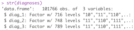
Of interest are 3 fields: diag_1, diag_2, diag_3. These 3 features are numerical representations of patient diagnoses. Each patient can have up to 3 diagnoses recorded. If we sum all the unique levels for all 3 sets, we end up with a lot of levels. Remember, even though these are numerical representations of diagnoses, they are still diagnoses and cannot be model as numerical data as the distance between two diagnoses doesn’t mean anything. These all need to be dummied into there own column.
length(unique(diabetes$diag_1))
## [1] 717
length(unique(diabetes$diag_2))
## [1] 749
length(unique(diabetes$diag_3))
## [1] 790
The sum of all unique diagnoses is 2256. This means, in order to break out each diagnosis into its own column, we need an additional 2256 new columns on top of our original 50.
OK, let’s finish cleaning up the data. We’re going to drop non-predictive features, replace interrogation marks with NAs and fix the outcome variable to a binary value.
# drop useless variables
diabetes <- subset(diabetes,select=-c(encounter_id, patient_nbr))

# transform all "?" to 0s
diabetes[diabetes == "?"] <- NA

# remove zero variance - ty James http://stackoverflow.com/questions/8805298/quickly-remove-zero-variance-variables-from-a-data-frame
diabetes <- diabetes[sapply(diabetes, function(x) length(levels(factor(x,exclude=NULL)))>1)]

# prep outcome variable to those readmitted under 30 days
diabetes$readmitted <- ifelse(diabetes$readmitted == "<30",1,0)

outcomeName <- 'readmitted'
Now, let’s prepare the data two ways: a common approach using dummy variables for our factors, and another using feature hashing.
Using Dummy Variables
Here we use caret’s dummyVars function to make our dummy column (see my walkthrough for more details on this great function). Be warned, you will need at least 2 gigabytes of free live memory on your system for this to work!
diabetes_dummy <- diabetes
# warning will need 2GB at least free memory
require(caret)
dmy <- dummyVars(" ~ .", data = diabetes_dummy)
diabetes_dummy <- data.frame(predict(dmy, newdata = diabetes_dummy))
After all this preparation work, we end up with a fairly wide data space with 2462 features/columns:
dim(diabetes_dummy)
## [1] 101766 2462
We’ll use cv.glmnet to model our data as it supports sparse matrices (this also works great with XGBoost).
# change all NAs to 0
diabetes_dummy[is.na(diabetes_dummy)] <- 0
# split the data into training and testing data sets
set.seed(1234)
split <- sample(nrow(diabetes_dummy), floor(0.5*nrow(diabetes_dummy)))
objTrain <-diabetes_dummy[split,]
objTest <- diabetes_dummy[-split,]

predictorNames <- setdiff(names(diabetes_dummy),outcomeName)

# cv.glmnet expects a matrix
library(glmnet)
# straight matrix model not recommended - works but very slow, go with a sparse matrix
# glmnetModel <- cv.glmnet(model.matrix(~., data=objTrain[,predictorNames]), objTrain[,outcomeName],
#             family = "binomial", type.measure = "auc")

glmnetModel <- cv.glmnet(sparse.model.matrix(~., data=objTrain[,predictorNames]), objTrain[,outcomeName],
                         family = "binomial", type.measure = "auc")
glmnetPredict <- predict(glmnetModel,sparse.model.matrix(~., data=objTest[,predictorNames]), s="lambda.min")
Let’s look at the AUC (Area under the curve) so we can compare this approach with the feature-hashed one:
auc(objTest[,outcomeName], glmnetPredict)
## [1] 0.6480986
Using Feature Hashing
Now for the fun part, remember that wide data set we just modeled? Well, by using feature hashing, we don’t have to do any of that work; we just feed the data set with its factor and character features directly into the model. The code is based on both a kaggle competition and Wush Wu’s package readme on GitHub.com.
The hashed.model.matrix function takes a hash.size value. This is a critical piece. Depending on the size of your data you may need to adjust this value. I set it here to 2^12, but if you try a larger value, it will handle more variables (i.e. unique values). On the other hand, if you try a smaller value, you risk having memory collisions and loss of data. It is something you have to experiment with.
diabetes_hash <- diabetes
predictorNames <- setdiff(names(diabetes_hash),outcomeName)

# change all NAs to 0
diabetes_hash[is.na(diabetes_hash)] <- 0

set.seed(1234)
split <- sample(nrow(diabetes_hash), floor(0.5*nrow(diabetes_hash)))
objTrain <-diabetes_hash[split,]
objTest <- diabetes_hash[-split,]

library(FeatureHashing)
objTrain_hashed = hashed.model.matrix(~., data=objTrain[,predictorNames], hash.size=2^12, transpose=FALSE)
objTrain_hashed = as(objTrain_hashed, "dgCMatrix")
objTest_hashed = hashed.model.matrix(~., data=objTest[,predictorNames], hash.size=2^12, transpose=FALSE)
objTest_hashed = as(objTest_hashed, "dgCMatrix")

library(glmnet)
glmnetModel <- cv.glmnet(objTrain_hashed, objTrain[,outcomeName],
                     family = "binomial", type.measure = "auc")
Let’s see how this version scored:
glmnetPredict <- predict(glmnetModel, objTest_hashed, s="lambda.min")
auc(objTest[,outcomeName], glmnetPredict)
## [1] 0.6475847
Practically the same score as prepping the data yourself but with half the work and a much smaller memory footprint.
Note: This subject and code was inspired by a Kaggle.com competition: Avazu - Click-Through Rate Prediction. More precisely by the following thread. I have used feature hashing in Python via sklearn’s preprocessing.OneHotEncoder and feature_extraction.FeatureHasher but these approaches aren’t as common in R. I hope this is changing with the arrival of great packages such as Wu’s. Many thanks to Wu and all Kagglers!!
# get data ----------------------------------------------------------------
# UCI Diabetes 130-US hospitals for years 1999-2008 Data Set
# https://archive.ics.uci.edu/ml/machine-learning-databases/00296/
require(RCurl)
binData <- getBinaryURL("https://archive.ics.uci.edu/ml/machine-learning-databases/00296/dataset_diabetes.zip",
                    ssl.verifypeer=FALSE)

conObj <- file("dataset_diabetes.zip", open = "wb")
writeBin(binData, conObj)
# don't forget to close it
close(conObj)

# open diabetes file
files <- unzip("dataset_diabetes.zip")
diabetes <- read.csv(files[1], stringsAsFactors = FALSE)

# quick look at the data
str(diabetes)

# drop useless variables
diabetes <- subset(diabetes,select=-c(encounter_id, patient_nbr))

# transform all "?" to 0s
diabetes[diabetes == "?"] <- NA

# remove zero variance - ty James http://stackoverflow.com/questions/8805298/quickly-remove-zero-variance-variables-from-a-data-frame
diabetes <- diabetes[sapply(diabetes, function(x) length(levels(factor(x,exclude=NULL)))>1)]

# prep outcome variable to those readmitted under 30 days
diabetes$readmitted <- ifelse(diabetes$readmitted == "<30",1,0)

# generalize outcome name
outcomeName <- 'readmitted'

# large factors to deal with
length(unique(diabetes$diag_1))
length(unique(diabetes$diag_2))
length(unique(diabetes$diag_3))

# dummy var version -------------------------------------------------------
diabetes_dummy <- diabetes
# alwasy a good excersize to see the length of data that will need to be transformed
# charcolumns <- names(diabetes_dummy[sapply(diabetes_dummy, is.character)])
# for (thecol in charcolumns)
#         print(paste(thecol,length(unique(diabetes_dummy[,thecol]))))

# warning will need 2GB at least free memory
require(caret)
dmy <- dummyVars(" ~ .", data = diabetes_dummy)
diabetes_dummy <- data.frame(predict(dmy, newdata = diabetes_dummy))

# many features
dim(diabetes_dummy)

# change all NAs to 0
diabetes_dummy[is.na(diabetes_dummy)] <- 0

# split the data into training and testing data sets
set.seed(1234)
split <- sample(nrow(diabetes_dummy), floor(0.5*nrow(diabetes_dummy)))
objTrain <-diabetes_dummy[split,]
objTest <- diabetes_dummy[-split,]

predictorNames <- setdiff(names(diabetes_dummy),outcomeName)

# cv.glmnet expects a matrix
library(glmnet)
# straight matrix model not recommended - works but very slow, go with a sparse matrix
# glmnetModel <- cv.glmnet(model.matrix(~., data=objTrain[,predictorNames]), objTrain[,outcomeName],
#             family = "binomial", type.measure = "auc")

glmnetModel <- cv.glmnet(sparse.model.matrix(~., data=objTrain[,predictorNames]), objTrain[,outcomeName],
                         family = "binomial", type.measure = "auc")
glmnetPredict <- predict(glmnetModel,sparse.model.matrix(~., data=objTest[,predictorNames]), s="lambda.min")

# dummy version score:
auc(objTest[,outcomeName], glmnetPredict)

# feature hashed version -------------------------------------------------
diabetes_hash <- diabetes
predictorNames <- setdiff(names(diabetes_hash),outcomeName)

# change all NAs to 0
diabetes_hash[is.na(diabetes_hash)] <- 0

set.seed(1234)
split <- sample(nrow(diabetes_hash), floor(0.5*nrow(diabetes_hash)))
objTrain <-diabetes_hash[split,]
objTest <- diabetes_hash[-split,]

library(FeatureHashing)
objTrain_hashed = hashed.model.matrix(~., data=objTrain[,predictorNames], hash.size=2^12, transpose=FALSE)
objTrain_hashed = as(objTrain_hashed, "dgCMatrix")
objTest_hashed = hashed.model.matrix(~., data=objTest[,predictorNames], hash.size=2^12, transpose=FALSE)
objTest_hashed = as(objTest_hashed, "dgCMatrix")

library(glmnet)
glmnetModel <- cv.glmnet(objTrain_hashed, objTrain[,outcomeName],
                     family = "binomial", type.measure = "auc")
# hashed version score:
glmnetPredict <- predict(glmnetModel, objTest_hashed, s="lambda.min")
auc(objTest[,outcomeName], glmnetPredict)
Manuel Amunategui - Follow me on Twitter: @amunategui